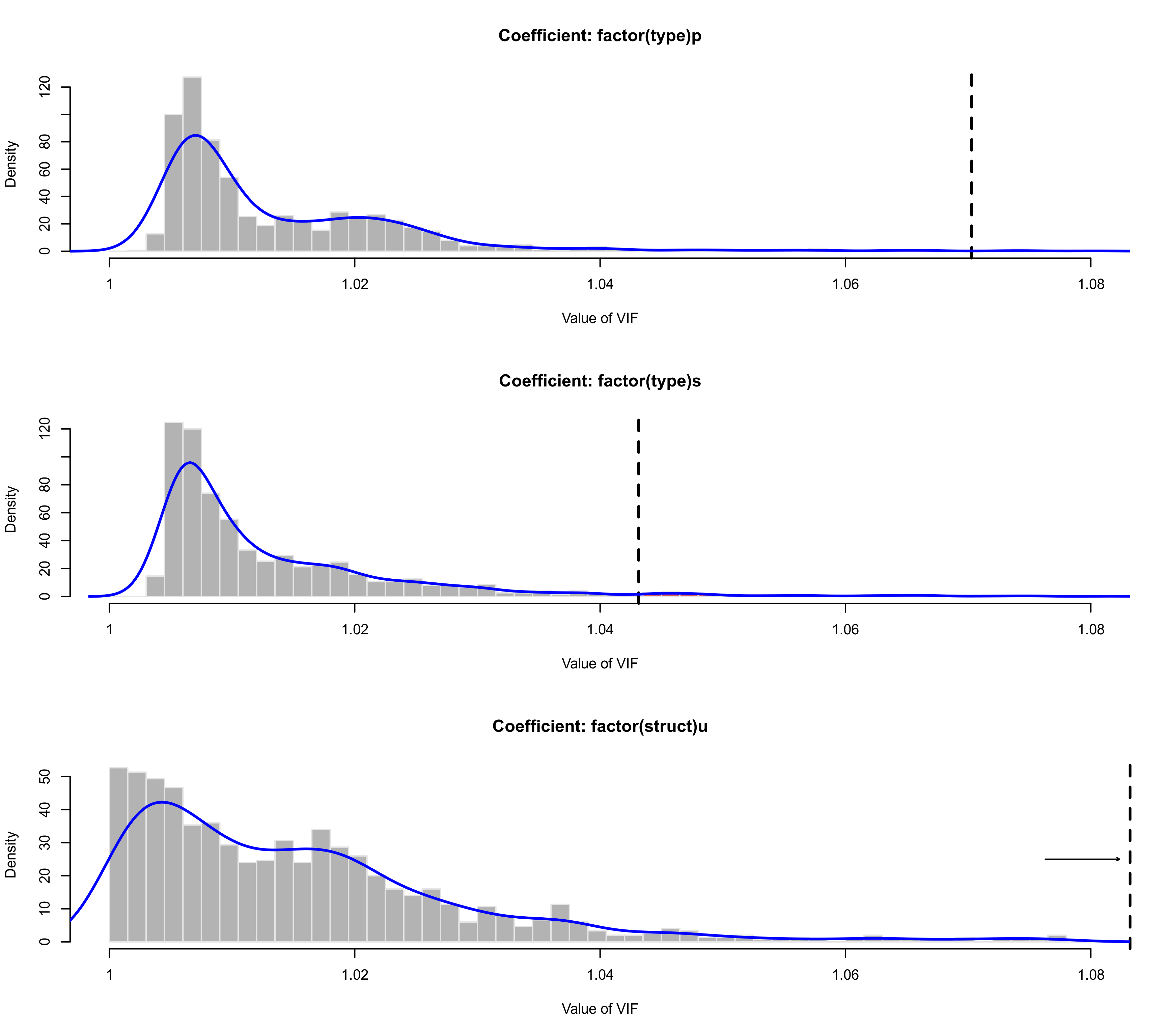
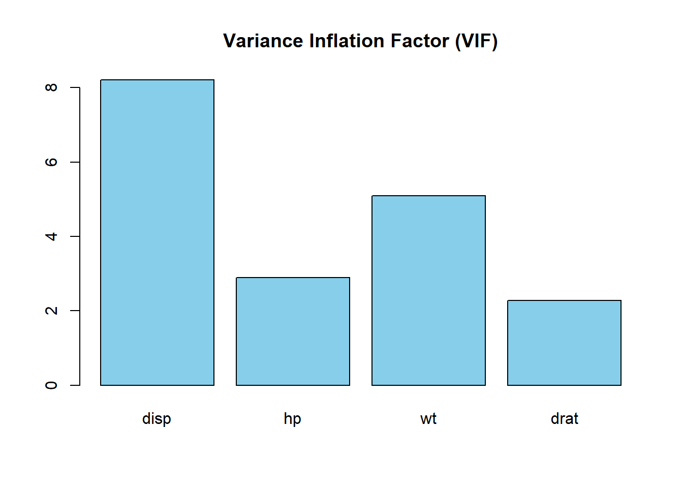
The Variance Inflation Factor (VIF) is a statistical diagnostic used to detect multicollinearity in a multiple linear regression model. It measures how much the variance of an estimated regression coefficient increases when your predictors are correlated. High VIF values indicate that redundant information exists among independent variables, which can make model estimates unstable and difficult to interpret.
In the world of statistical modeling and predictive analytics, the accuracy of a regression model depends heavily on the quality and independence of its input variables. While we often focus on the relationship between the independent variables and the dependent variable, the relationships between the independent variables themselves—known as multicollinearity—can silently undermine the reliability of the entire analysis. As we navigate the complex data landscapes of 2026, understanding tools like the Variance Inflation Factor remains fundamental for researchers, data scientists, and analysts who require robust, interpretable results.
The Problem of Multicollinearity in Regression
To appreciate the Variance Inflation Factor, one must first understand the phenomenon it is designed to diagnose: multicollinearity. In an ideal multiple linear regression scenario, each independent variable (predictor) provides unique, incremental information about the dependent variable (outcome). However, in many real-world datasets, independent variables are correlated with one another.
When two or more variables are highly correlated, they are essentially providing overlapping information. This redundancy makes it difficult for the Ordinary Least Squares (OLS) algorithm to isolate the individual effect of each predictor. Mathematically, this manifests as an increase in the standard errors of the regression coefficients. Large standard errors mean that the coefficients are estimated with low precision. A variable that is actually a significant predictor might appear statistically insignificant because its standard error has been "inflated" by its correlation with other variables.
This instability is particularly problematic when the goal of the regression is inference rather than just prediction. If you need to explain how much a specific change in $X$ influences $Y$, multicollinearity can lead to nonsensical results, such as coefficients with the "wrong" sign (e.g., a positive correlation showing up as a negative coefficient in the model) or results that change drastically with minor adjustments to the data.
Defining the Variance Inflation Factor (VIF)
The Variance Inflation Factor provides a numerical index that quantifies how much the variance of an estimated regression coefficient is increased due to collinearity with other predictors in the model. The term "inflation" is literal here: it describes the factor by which the variance of the coefficient is larger than it would be if the predictor were completely uncorrelated with the other independent variables.
The VIF for a specific predictor $X_j$ is calculated using the following logical steps:
- Isolate the Predictor: Choose one independent variable ($X_j$) from the model.
- Run an Auxiliary Regression: Perform a linear regression where $X_j$ is the dependent variable and all other independent variables in the original model are the predictors.
- Identify the R-squared: Calculate the $R^2$ value (coefficient of determination) from this auxiliary regression. Let’s call this $R^2_j$.
- Calculate VIF: Use the formula: $VIF_j = 1 / (1 - R^2_j)$.
The denominator $(1 - R^2_j)$ is also known as the Tolerance. If $R^2_j$ is high (close to 1), it means $X_j$ can be almost perfectly predicted by the other variables. This results in a very small tolerance and, consequently, a very high VIF. Conversely, if $X_j$ is independent of the others, $R^2_j$ will be close to 0, and the VIF will be close to 1.

Interpreting VIF Thresholds and Scores
Interpreting VIF scores requires a balance between statistical rigor and the practical context of the research. Because VIF starts at 1 and has no upper bound, analysts typically use standardized thresholds to decide when multicollinearity has become a "problem" that requires intervention.
- VIF = 1: This indicates no correlation between the predictor and the other independent variables. The variance of the coefficient is not inflated at all.
- VIF between 1 and 5: This suggests moderate correlation, but it is generally considered acceptable in most social science and business contexts. The estimates are still relatively stable.
- VIF > 5: Many researchers use 5 as a conservative cutoff. At this level, multicollinearity is becoming significant enough that it might start masking the true relationships in the data.
- VIF > 10: This is the most common "rule of thumb" for high multicollinearity. A VIF of 10 means the variance of the coefficient is 10 times larger than it should be. At this point, the regression coefficients are likely unstable, and the p-values may be misleading.
It is important to note that these thresholds are not absolute laws. In some fields, like econometrics or physics, where high precision is required, a VIF of 3 might be considered too high. In other contexts, such as models containing polynomial terms (like $X$ and $X^2$) or interaction terms ($X \times Z$), high VIF values are mathematically expected and do not necessarily invalidate the model's findings.
The Mathematical Impact on Model Reliability
High VIF values have a direct impact on the quality of a regression model. To understand why, we look at the formula for the variance of a regression coefficient $\beta_j$:
$Var(\beta_j) = \frac{\sigma^2}{\sum(x_{ij} - \bar{x}_j)^2} \times VIF_j$
In this equation, $\sigma^2$ represents the error variance of the model. The VIF acts as a multiplier. If the VIF is 10, the variance of your estimate is 10 times larger than the ideal case. Since the standard error is the square root of the variance, a VIF of 10 results in a standard error that is approximately 3.16 times larger ($\sqrt{10}$).
This inflation directly affects the t-statistic, which is calculated by dividing the coefficient by its standard error. As the standard error increases, the t-statistic decreases. Consequently, the p-value increases, often pushing it above the standard 0.05 threshold for statistical significance. This leads to Type II errors: failing to detect a real relationship because the "noise" of multicollinearity has drowned out the signal.
Furthermore, high VIF values lead to wider confidence intervals. A wide confidence interval means we are less certain about the true value of the effect. In a business forecasting scenario, this could mean the difference between predicting a 5% increase in sales with high confidence and predicting a range between -10% and +20%, which is essentially useless for decision-making.
Comparison of Multicollinearity Diagnostics
While VIF is the most popular diagnostic tool, it is often used alongside other measures to get a complete picture of the data structure. The following table compares VIF with other common metrics used in 2026.
| Metric | Purpose | Threshold for Concern | Pros / Cons |
|---|---|---|---|
| VIF | Measures variance inflation for each individual predictor. | > 5 or > 10 | Easy to interpret; identifies which specific variable is the problem. |
| Tolerance | Reciprocal of VIF ($1/VIF$). | < 0.1 or < 0.2 | Directly shows the percentage of unique variance; redundant if VIF is used. |
| Correlation Matrix | Measures pairwise linear relationships between two variables. | > 0.8 or 0.9 | Simple to calculate; fails to detect "multivariate" collinearity (3+ variables). |
| Condition Index | Measures the overall "ill-conditioning" of the data matrix. | > 30 | Provides a global view of model stability; mathematically complex to explain. |
| Eigenvalues | Decomposition of the correlation matrix. | Near 0 | Deep mathematical insight; difficult for non-statisticians to interpret. |
Practical Strategies for Managing High VIF
If your model reports VIF values that exceed your chosen threshold, you must decide how to proceed. Simply ignoring high VIF can lead to fragile models that fail when applied to new data. Here are the most effective strategies for remediation:
1. Removing Redundant Variables
The most straightforward solution is to identify which variables are highly correlated and remove one of them. For example, if you are modeling house prices and include both "Total Square Footage" and "Number of Rooms," these are likely to have a very high VIF. Removing the one that is less theoretically relevant often resolves the issue without losing much predictive power.
2. Combining Variables (Feature Engineering)
Instead of dropping data, you can merge correlated variables into a single index. If you have five different variables measuring "customer satisfaction," you could average them into a "Composite Satisfaction Score." This reduces the number of predictors and eliminates the internal correlation while preserving the information from all five original inputs.
3. Increasing the Sample Size
Multicollinearity is often a "small sample" problem. With a larger dataset, the standard errors naturally decrease. While this doesn't change the VIF (which is based on the correlation structure, not sample size), it can provide enough precision that the "inflated" variance is still small enough to allow for significant results.
4. Principal Component Analysis (PCA)
PCA is a data reduction technique that transforms a set of correlated variables into a smaller set of uncorrelated variables called Principal Components. By using these components in your regression instead of the raw variables, you guarantee a VIF of exactly 1 for every predictor. The downside is that PCA components are harder to interpret than the original variables.
5. Regularization (Ridge and Lasso Regression)
In modern data science, regularization is a preferred method for handling multicollinearity. Ridge Regression adds a penalty term to the OLS equation that shrinks the coefficients. While this introduces a small amount of bias, it significantly reduces the variance (the "inflation"), leading to more reliable predictions. Lasso Regression goes a step further by shrinking some coefficients all the way to zero, effectively performing automatic variable selection.
Frequently Asked Questions
Can I have a high VIF and still have a good model?
Yes, particularly if your primary goal is prediction rather than inference. If you only care about accurately predicting the dependent variable and the correlation structure of the predictors remains the same in the future, high VIF might not be an issue. Additionally, high VIF is expected and often harmless in models with polynomial or interaction terms, provided the variables are centered.
Does a low VIF guarantee that my model is accurate?
No. A low VIF only means that multicollinearity is not an issue. Your model could still suffer from omitted variable bias, non-linear relationships, heteroscedasticity, or poor data quality. VIF is a diagnostic for one specific problem, not a certificate of overall model validity.
How do I calculate VIF in common software like R or Python?
In Python, the most common approach is using the variance_inflation_factor function from the statsmodels.stats.outliers_influence library. In R, the vif() function from the car package is the standard tool. Both require you to first define your independent variable matrix.
Is VIF relevant for non-linear models like Logistic Regression?
While VIF is most commonly associated with linear regression, the concept of multicollinearity applies to logistic regression as well. You can calculate VIF for logistic regression by treating the independent variables as if they were in a linear model, as the correlation between predictors is independent of the distribution of the outcome variable.
Why is 10 the most common threshold for VIF?
The threshold of 10 corresponds to an $R^2$ of 0.90 in the auxiliary regression. It is a somewhat arbitrary "rule of thumb" that has become a standard in the industry. However, many modern practitioners prefer a stricter threshold of 5 (corresponding to an $R^2$ of 0.80) to ensure higher model stability.
Recommendation for Practical Application
When performing regression analysis, you should calculate the Variance Inflation Factor as a standard part of your diagnostic workflow. Do not treat VIF thresholds as absolute "pass/fail" markers; instead, use them as a signal to investigate your data more deeply. If you encounter a high VIF, start by checking for logical redundancies in your variables—such as including the same measurement in different units.
If the high VIF is caused by variables that are both theoretically essential, consider using Ridge Regression or Elastic Net regularization. These methods allow you to keep all your predictors while mathematically mitigating the instability caused by variance inflation. By 2026 standards, a robust model is one that balances predictive power with structural integrity, and monitoring VIF is a critical step in achieving that balance.
For more technical details on the underlying linear algebra of VIF, the NIST Engineering Statistics Handbook and the documentation for the Statsmodels library provide extensive resources for implementation and theory.
Image Gallery
Select an image to open it in a new tab.

Mateo Castillo
Decentralized Finance and E-Payments Strategist
