Predictive Analytic Techniques Explained: A Comprehensive Guide to Algorithms and Applications
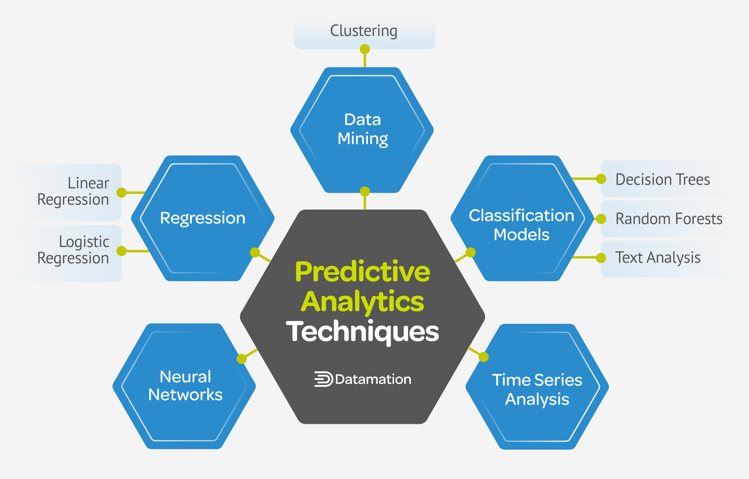
Predictive analytic techniques use statistical algorithms, historical data, and machine learning models to forecast future outcomes, estimate continuous numerical values, or classify categorical behaviors. By analyzing underlying patterns in existing datasets, organizations assess operational risks, optimize inventory allocation, detect fraud, and personalize user experiences before outcomes materialize.
Fundamentals of Predictive Analytics
Predictive analytics sits at the intersection of mathematical statistics, computer science, and domain expertise. To evaluate predictive techniques effectively, it is helpful to place them within the broader business analytics framework:
- Descriptive Analytics: Examines historical metrics to summarize what occurred over a defined period (e.g., monthly revenue reporting).
- Diagnostic Analytics: Evaluates relationships in historical data to understand why an outcome occurred (e.g., root-cause analysis of customer churn).
- Predictive Analytics: Uses historical observations and mathematical modeling to estimate the probability of future events or quantitative values (e.g., demand forecasting).
- Prescriptive Analytics: Synthesizes predictive forecasts with optimization algorithms to recommend specific automated or operational actions (e.g., real-time dynamic pricing).
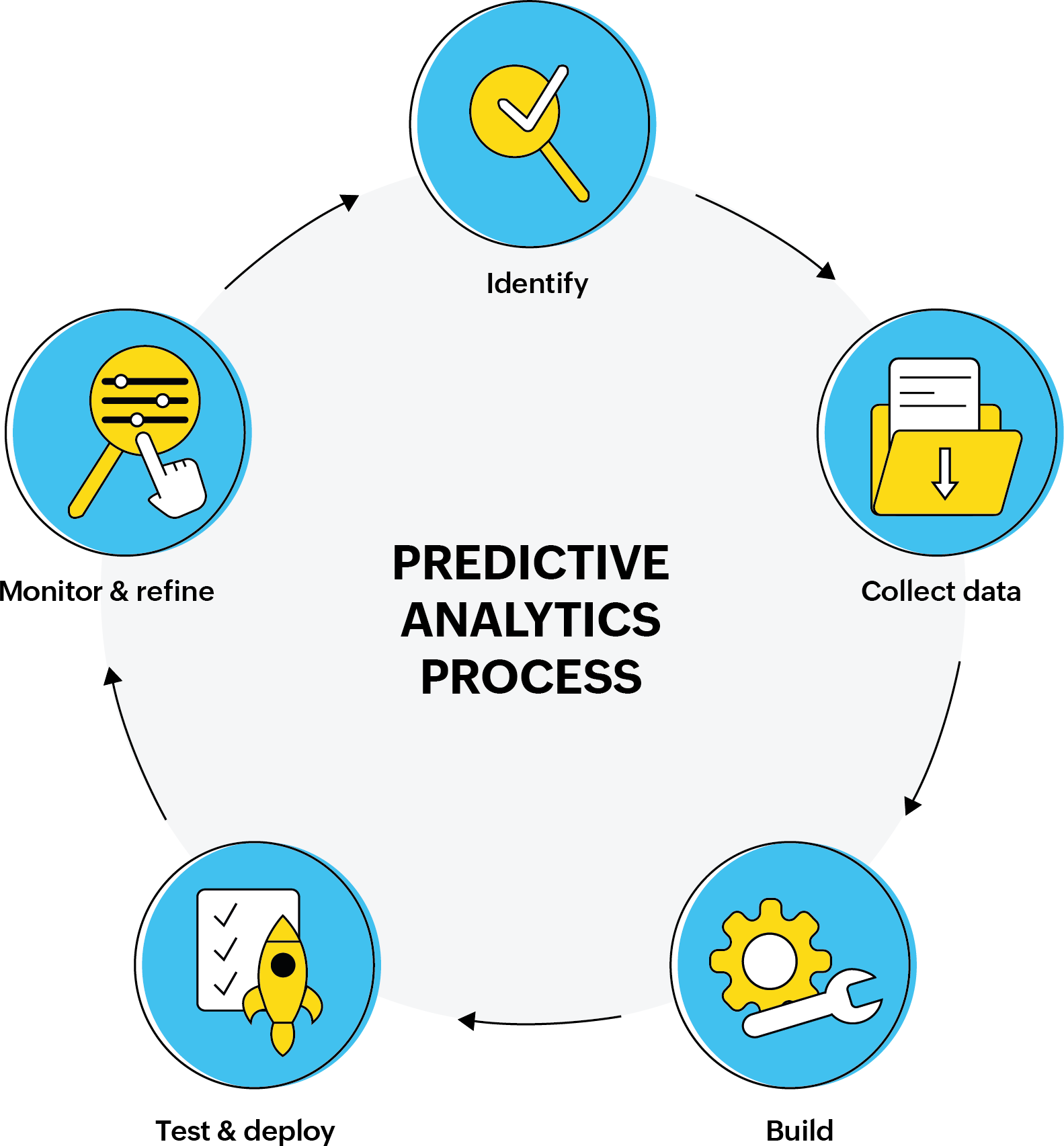
The Predictive Modeling Pipeline
Every predictive technique relies on a structured data processing workflow:
- Problem Definition: Formulating a clear target variable—such as estimating credit default probability or predicting equipment failure within 30 days.
- Data Acquisition and Ingestion: Gathering structured data (tabular databases) and unstructured data (text, sensor streams) from internal enterprise systems and external APIs.
- Data Preprocessing & Feature Engineering: Cleaning raw input data by imputing missing values, removing noise, handling outliers, normalizing numeric ranges, and transforming raw columns into predictive indicators (features).
- Model Training & Hyperparameter Tuning: Splitting data into training, validation, and testing subsets, then fitting algorithms on historical patterns while optimizing parameter configurations.
- Model Evaluation & Validation: Testing model generalizeability against unseen evaluation sets using standardized statistical metrics.
- Deployment & Continuous Monitoring: Deploying validated models into production environments (microservices, batch jobs) and monitoring performance against data drift over time.
Statistical Predictive Techniques
Statistical models form the bedrock of predictive analytics. These techniques emphasize mathematical interpretability, confidence intervals, and hypothesis testing.
Linear Regression and Regularized Variants
Linear regression models the direct mathematical relationship between a continuous dependent target variable ($y$) and one or more independent predictive features ($X$). The standard Ordinary Least Squares (OLS) method minimizes the sum of squared residuals between observed and predicted values.
$$\hat{y} = \beta_0 + \beta_1 x_1 + \beta_2 x_2 + \dots + \beta_p x_p$$
When handling datasets with high feature dimensions or strong multicollinearity (high correlation between input features), standard linear regression risks overfitting. Advanced regularized variants address this limitation:
- Ridge Regression ($L_2$ Regularization): Adds a penalty proportional to the square of the magnitude of the coefficients. This shrinks coefficients toward zero without forcing them entirely to zero, stabilizing models with correlated inputs.
- Lasso Regression ($L_1$ Regularization): Adds a penalty proportional to the absolute value of the coefficients. Lasso forces non-informative feature coefficients to exactly zero, performing built-in feature selection.
- ElasticNet: Combines $L_1$ and $L_2$ penalties to balance feature selection and coefficient stabilization, particularly useful when feature count exceeds sample size.
Logistic Regression
Despite its name, logistic regression is a classification technique used when the target variable is categorical—most commonly binary (e.g., fraud vs. non-fraud, churn vs. retention). Instead of outputting a raw continuous number, logistic regression uses the sigmoid (logit) activation function to map linear outputs into a bounded probability range between 0 and 1:
$$P(Y=1|X) = \frac{1}{1 + e^{-(\beta_0 + \beta^T X)}}$$
Logistic regression remains widely deployed in regulated industries such as healthcare and banking because coefficients directly represent the log-odds of an event occurring, making model decisions fully explainable to auditors.
Time Series Forecasting
Time series analysis processes sequence data ordered chronologically, isolating underlying temporal structures such as trends, seasonality, cyclical patterns, and random noise.
Time Series Component Breakdown: Raw Observation = Trend Component + Seasonal Pattern + Cyclical Variability + Irregular Noise
Key algorithms in statistical time series forecasting include:
- ARIMA (AutoRegressive Integrated Moving Average): Combines autoregressive terms (past values), differencing operations (to achieve stationarity), and moving average terms (past prediction errors). ARIMA is designed for univariate time series data without complex nested seasonality.
- SARIMAX: Extends ARIMA to incorporate explicit seasonal periods (e.g., quarterly spikes) and exogenous explanatory variables (external covariates like promotional spend).
- Exponential Smoothing (Holt-Winters): Applies exponentially decreasing weights to older observations while explicitly modeling trend and multiplicative or additive seasonality.

Machine Learning Predictive Techniques
Machine learning algorithms relax linear assumptions, allowing predictive pipelines to capture complex non-linear relationships, multi-way feature interactions, and large-scale data structures.
Decision Trees and Random Forests
Decision trees segment feature spaces by applying sequential, rule-based binary splits that maximize information gain or minimize node impurity (using metrics like Gini Impurity or Variance Reduction).
While individual decision trees are prone to overfitting, ensemble methods solve this by combining multiple decision trees:
- Random Forests: An ensemble technique using bootstrap aggregation (bagging). It trains hundreds of independent decision trees on random subsets of the data and random feature subsets. The final prediction aggregates outputs across all trees (majority voting for classification, mean averaging for regression). This significantly reduces prediction variance and prevents individual tree overfitting.
Gradient Boosting Machines (GBMs)
Gradient boosting constructs an ensemble of decision trees sequentially rather than independently. Each new tree focuses specifically on predicting the residual errors left unresolved by the preceding combined trees, using gradient descent to minimize a specified loss function.
Modern high-performance implementations include:
- XGBoost (Extreme Gradient Boosting): Incorporates regularization terms directly into the objective function, supports parallel tree construction, and handles missing data natively.
- LightGBM: Employs leaf-wise tree growth and histogram-based feature binning, reducing memory consumption and processing times on massive enterprise datasets.
- CatBoost: Optimized specifically for categorical features using ordered target encoding, reducing pre-processing overhead and data leakage.
Neural Networks and Deep Learning Models
Deep learning architectures utilize layered networks of artificial neurons to automatically discover complex feature representations directly from raw inputs.
Input Layer ---> Hidden Layers (Representation Learning) ---> Output Layer (Raw Features) (Dense / Convolutional / Recurrent) (Prediction)
- Feedforward Neural Networks (MLPs): Multi-Layer Perceptrons consisting of fully connected layers, used for complex non-linear tabular modeling.
- Recurrent Neural Networks (RNNs) and LSTMs: Networks equipped with internal memory gates, designed to evaluate sequential inputs such as long-term financial transactions or medical temporal telemetry.
- Transformers: Modern architectures using self-attention mechanisms to weigh relationships across sequential elements simultaneously. While pioneered for natural language processing, transformer architectures (e.g., Temporal Fusion Transformers) are increasingly applied to high-dimensional time-series forecasting.
Comparative Matrix of Predictive Techniques
Selecting the correct predictive algorithm depends on target data types, performance demands, latency constraints, and interpretability requirements.
| Predictive Technique | Target Variable Type | Primary Strengths | Notable Limitations | Common Practical Use Case |
|---|---|---|---|---|
| Linear Regression | Continuous Numerical | Highly interpretable, fast training, minimal compute footprint | Assumes linear relationships; sensitive to outliers | Real estate property valuation, revenue baseline estimation |
| Logistic Regression | Binary / Multinomial Categorical | Outputs direct probabilities, clear feature coefficients | Struggles with complex non-linear boundary limits | Credit default risk scoring, disease risk screening |
| ARIMA / SARIMAX | Continuous Sequential | Strong statistical baseline for chronological series | Requires stationary data; limited multi-step non-linear capacity | Quarterly utility demand forecasting, macro-economic metrics |
| Random Forest | Continuous or Categorical | Handles missing values well, robust against overfitting | Large model file sizes, slower real-time inference speed | Churn prediction, operational risk classification |
| Gradient Boosting (XGBoost) | Continuous or Categorical | State-of-the-art accuracy on structured tabular datasets | Requires careful hyperparameter tuning; prone to noise overfitting | E-commerce recommendation ranking, fraud detection |
| Deep Neural Networks | Any (Text, Image, Tabular, Time-Series) | Unrivaled performance on high-dimensional unstructured data | Requires massive training datasets and high GPU compute power | Predictive asset maintenance via audio/sensor streams |
Model Evaluation Metrics
A predictive model must be evaluated using metrics aligned with specific operational targets and business costs.
Confusion Matrix Overview: Actual Positive Actual Negative Predicted Positive: True Positive (TP) False Positive (FP) [Type I Error] Predicted Negative: False Negative (FN) True Negative (TN) [Type II Error]
Metrics for Regression Tasks
Regression metrics measure the distance between continuous predictions ($\hat{y}_i$) and actual target values ($y_i$):
- Mean Absolute Error (MAE): The average magnitude of absolute errors. It provides an intuitive metric in the original units of measurement: $$\text{MAE} = \frac{1}{n} \sum_{i=1}^{n} |y_i - \hat{y}_i|$$
- Root Mean Squared Error (RMSE): Penalizes larger errors more heavily by squaring residuals before averaging. It is sensitive to extreme outliers.
- R-Squared ($R^2$): Measures the proportion of variance in the dependent variable explained by the model relative to a simple mean baseline.
Metrics for Classification Tasks
For classification models, evaluating simple accuracy can be misleading when datasets are imbalanced (e.g., rare transaction fraud):
- Precision: $\frac{TP}{TP + FP}$ — Measures what fraction of positive predictions were actually correct. High precision is crucial when false alarms carry high operational costs.
- Recall (Sensitivity): $\frac{TP}{TP + FN}$ — Measures what fraction of actual positive instances were successfully identified. High recall is critical when missing a positive case carries severe consequences (e.g., medical diagnostics).
- F1-Score: The harmonic mean of Precision and Recall, providing a balanced single metric for class-imbalanced settings: $$\text{F1} = 2 \cdot \frac{\text{Precision} \cdot \text{Recall}}{\text{Precision} + \text{Recall}}$$
- ROC-AUC: Area under the Receiver Operating Characteristic curve. It measures the model's ability to discriminate between positive and negative classes across all possible probability thresholds.
Step-by-Step Implementation Framework
Deploying predictive techniques into production environments requires an enterprise-grade execution framework to ensure reliability and maintainability.
1. Problem Formulation and KPI Alignment
Translate business objectives into structured predictive objectives. Identify the precise prediction horizon (e.g., predicting 7 days vs. 90 days in advance) and establish performance baselines against existing manual or rule-based heuristics.
2. Data Engineering & Sanitization
Establish secure data ingestion pipelines. Clean incoming features, handle missing data using domain-appropriate techniques (such as forward-filling time series or median imputation for tabular data), and convert raw metrics into structured datasets. Split data strictly along time boundaries for sequence problems to avoid data leakage.
3. Model Building & Validation
Train multiple candidate model architectures. Use cross-validation procedures—such as stratified $K$-fold for classification or rolling time-series split cross-validation for sequential tasks—to evaluate model generalization without exposing validation data to training steps.
4. Operational Deployment
Package trained model artifacts alongside input preprocessing pipelines into executable containers or microservices. Depending on operational requirements, deploy the pipeline as a real-time REST API endpoint or as an asynchronous batch processing job. Enterprise standards for model packaging can be referenced through the Open Neural Network Exchange (ONNX) standard.
5. Governance, Monitoring, and Drift Management
Once live, continuously log input feature distributions and prediction outputs. Monitor for two key operational degradation vectors:
- Data Drift (Covariate Shift): Changes in input data distributions over time (e.g., macro-economic shifts altering consumer spending behaviors).
- Concept Drift: Changes in the underlying statistical relationship between features and the target variable (e.g., evolving fraud tactics altering transaction patterns).
Common Pitfalls and Technical Limitations
Building effective predictive models requires avoiding several recurring technical implementation errors:
Data Leakage
Data leakage occurs when information from the target variable or future test periods inadvertently leaks into training features during preprocessing or scaling. Common examples include fitting feature scalers on the entire dataset prior to train-test splitting, or including feature columns calculated using future time windows.
Overfitting vs. Underfitting
- Overfitting: Occurs when an overly complex model learns noise and specific instances from training data rather than underlying generalized patterns. It manifests as high training accuracy paired with poor test performance. Address overfitting by using regularization, pruning decision trees, or increasing training sample sizes.
- Underfitting: Occurs when an overly simplistic model cannot capture structural relationships in data. Address underfitting by introducing non-linear transformations, engineering richer features, or choosing a higher-capacity algorithm.
The Interpretability-Performance Trade-off
Highly complex models like deep neural networks and dense ensemble boosters often deliver top predictive accuracy, but operate as "black boxes." In contrast, simpler linear models provide clear mathematical interpretability at the expense of potential capacity limitations.
To bridge this gap in regulated environments, data teams deploy model-agnostic explainability frameworks, such as:
- SHAP (SHapley Additive exPlanations): Calculates Shapley values from cooperative game theory to quantify the exact feature contribution of every input to a given individual prediction.
- LIME (Local Interpretable Model-agnostic Explanations): Builds localized surrogate linear models around specific predictions to explain how the complex model behaves in that local feature space.
Frequently Asked Questions
What is the difference between machine learning and predictive analytics?
Predictive analytics is a broad domain focused on forecasting future events or quantitative values using historical data. Machine learning is a subset of artificial intelligence providing specific non-linear, data-driven algorithms (such as Random Forests and Neural Networks) used within predictive analytics pipelines.
How do I choose the best predictive technique for my dataset?
Start with dataset characteristics and operational requirements. Use statistical linear or logistic regression if complete model transparency is mandated by regulators. Use ensemble methods like XGBoost or Random Forests for tabular business data with complex non-linear feature interactions. Use deep learning or transformer architectures when dealing with high-dimensional unstructured inputs like text, audio, image telemetry, or long continuous sequences.
Why is data preprocessing critical in predictive modeling?
Predictive algorithms rely directly on mathematical operations. Unhandled missing values, unscaled numeric features, extreme data noise, or misformatted temporal inputs degrade algorithm convergence and yield inaccurate statistical parameters. Thorough data sanitization prevents propagation of input errors into model outputs.
What is concept drift and how does it affect predictive accuracy?
Concept drift occurs when the true mathematical relationship between input features and target variables changes over time. For example, consumer purchase behaviors established during historical baselines may change following macroeconomic shifts, rendering older predictive models inaccurate. Organizations mitigate concept drift through automated data logging, scheduled retrain cycles, and continuous performance auditing.
Can predictive analytic techniques work with small datasets?
Yes, provided the chosen algorithm aligns with dataset size constraints. Complex deep neural networks require large datasets to generalize properly, but statistical models like Linear Regression, Ridge/Lasso, Naive Bayes, or smaller Decision Trees perform reliably on limited samples when paired with robust cross-validation techniques.
Strategic Recommendations for Implementation
To successfully deploy predictive analytics within your operational workflows, follow these pragmatic steps:
- Establish Clear Baseline Models: Always build a simple baseline model—such as a linear regression or historical average—before training complex ensemble models or deep networks. Evaluate whether added architectural complexity yields actionable business value.
- Prioritize Data Engineering: Model accuracy relies on high-quality input features. Focus initial project resources on cleaning data sources, building stable ingestion pipelines, and creating domain-specific features.
- Implement Robust Validation Splits: Avoid standard random splits when working with sequence data. Use temporal time-series splits to evaluate how models perform under realistic forward-looking operational conditions.
- Plan for Long-Term Model Governance: Deploy active telemetry tools alongside model microservices to measure latency, monitor input drift, and trigger continuous retraining routines when model outputs fall below established statistical thresholds.
Image Gallery
Select an image to open it in a new tab.






Declan O'Connor
Higher Education and Campus Culture Reporter
