
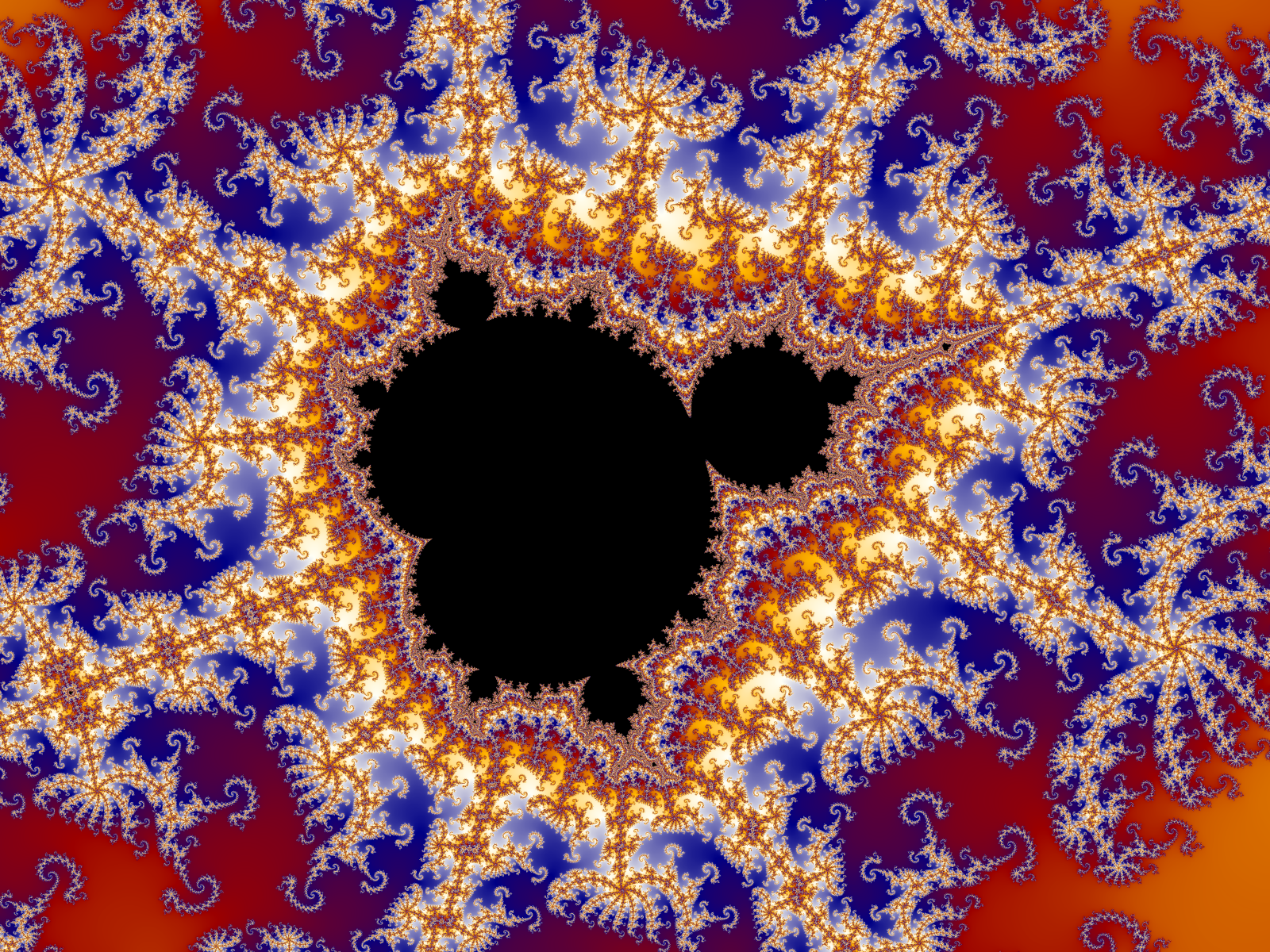
The Mandelbrot set is a famous mathematical structure in fractal geometry defined as the set of complex numbers $c$ for which the iterative function $z_{n+1} = z_n^2 + c$ does not tend toward infinity when starting from $z_0 = 0$. When plotted on the complex plane, it forms an intricately detailed boundary exhibiting infinite complexity and self-similarity.
What Is the Mandelbrot Set?
At its core, the Mandelbrot set is a visual map of mathematical stability. Named after the mathematician Benoit Mandelbrot, who popularized its study in 1980 while working at IBM's Thomas J. Watson Research Center, this geometric object is generated by a surprisingly simple mathematical rule.
Despite being defined by an equation containing only addition and basic multiplication, the boundary of the set produces infinitely intricate shapes, spiral patterns, smaller replicas of itself, and organic visual structures. If you zoom into any section of its border, new geometric features continue to emerge regardless of how deeply you magnify the image.
To create the visualization, every point on a two-dimensional grid—representing the complex number plane—is tested through a repetitive mathematical process called iteration. Points that remain bounded (they stay small and never blow up to infinity) belong to the Mandelbrot set itself. Points that grow infinitely large do not belong to the set. In standard fractal images, the points within the set are typically colored solid black, while the points outside the set are colored according to how quickly their values escaped toward infinity.
The Core Mathematics Behind the Set
Understanding the Mandelbrot set requires examining three mathematical concepts: complex numbers, iteration, and numerical boundedness.
Understanding Complex Numbers and the Complex Plane
In standard algebra, numbers sit on a one-dimensional line containing negative numbers, zero, and positive numbers. Complex numbers expand this system into two dimensions by introducing the imaginary unit, denoted as $i$, which is defined as the square root of negative one ($i^2 = -1$).
A complex number $c$ is written in the form:
$$c = a + bi$$
In this expression:
- $a$ represents the real part, plotted along the horizontal x-axis.
- $b$ represents the imaginary part, plotted along the vertical y-axis.
When we view the complex plane as a two-dimensional grid, every single pixel on a display screen can correspond to a specific complex coordinate $c = a + bi$. For example, the center of the main body of the Mandelbrot set sits near the point $(-0.75, 0)$, corresponding to the complex number $-0.75 + 0i$.
The Iterative Formula: $z_{n+1} = z_n^2 + c$
The engine behind the Mandelbrot set is the recursive function:
$$z_{n+1} = z_n^2 + c$$
In this sequence:
- $c$ is the fixed position (complex number) on the grid being evaluated.
- $z$ is a variable number that changes with every iteration step ($n$).
- The process always begins with $z_0 = 0$.
To evaluate a specific point $c$, you perform the arithmetic step-by-step:
- Step 0: $z_0 = 0$
- Step 1: $z_1 = (z_0)^2 + c = 0^2 + c = c$
- Step 2: $z_2 = (z_1)^2 + c = c^2 + c$
- Step 3: $z_3 = (z_2)^2 + c = (c^2 + c)^2 + c$
This loop repeats indefinitely, feeding the output of the previous step back in as the input for the next step.
Numerical Example 1: A Point Inside the Set
Let us test $c = 0$:
- $z_0 = 0$
- $z_1 = 0^2 + 0 = 0$
- $z_2 = 0^2 + 0 = 0$
The value stays at $0$ forever. Because it never grows or escapes to infinity, $c = 0$ is inside the Mandelbrot set.
Numerical Example 2: Another Point Inside the Set
Let us test $c = -1$:
- $z_0 = 0$
- $z_1 = 0^2 + (-1) = -1$
- $z_2 = (-1)^2 + (-1) = 1 - 1 = 0$
- $z_3 = 0^2 + (-1) = -1$
The sequence oscillates indefinitely between $0$ and $-1$. Because the numbers remain small and bounded, $c = -1$ is inside the Mandelbrot set.
Numerical Example 3: A Point Outside the Set
Let us test $c = 1$:
- $z_0 = 0$
- $z_1 = 0^2 + 1 = 1$
- $z_2 = 1^2 + 1 = 2$
- $z_3 = 2^2 + 1 = 5$
- $z_4 = 5^2 + 1 = 26$
The values grow rapidly toward infinity. Therefore, $c = 1$ is outside the Mandelbrot set.
The Boundedness Test and the Escape Radius
Mathematically, how do we know for certain whether a sequence will head to infinity without running the calculation forever?
This is governed by the Escape Radius Theorem. In complex analysis, the magnitude (or distance from the origin) of a complex number $z = x + iy$ is calculated using the Pythagorean formula:
$$|z| = \sqrt{x^2 + y^2}$$
It is mathematically proven that if the distance $|z_n|$ ever exceeds $2$ for any step $n$ in the iteration sequence, the values are guaranteed to escape to infinity. Once $|z_n| > 2$, the term $(z_n)^2$ dominates the addition of $c$, causing exponential divergence.
Therefore, computer algorithms do not need to iterate infinitely. They simply compute values of $z_n$ up to a designated maximum limit (such as 500 or 1,000 iterations). If $|z_n|$ exceeds 2 before reaching the maximum iteration count, the calculation stops, marking the point $c$ as outside the set. If the calculation reaches the maximum limit without $|z_n|$ exceeding 2, the point $c$ is classified as inside the set.

Key Anatomy and Geometric Features
When rendered visually, the Mandelbrot set exhibits distinct structural regions, each possessing distinct mathematical properties.
Complex Plane Representation y (Imaginary) ^ | Period-3 Bulb | (Top) .---. | .---. / \|/ \ Period-2 Bulb +--| Main Cardioid |--+ Antenna / Spike (-1.0, 0) | \ /|\ / | (-2.0, 0) <---------------+--'-'---|'-'---+---> x (Real) | .---. | .---. / /|\ \ '-----' | '-----' | Period-3 Bulb | (Bottom) v
The Main Cardioid
The largest central body of the Mandelbrot set is a heart-shaped region known as the main cardioid. Mathematically, any complex number $c$ lying inside this cardioid causes the iteration sequence to converge toward a single stable fixed point rather than oscillating or escaping.
The boundary of the main cardioid can be defined parametrically using complex numbers derived from Euler's formula:
$$c = \frac{1}{2}e^{i\theta} - \frac{1}{4}e^{2i\theta}$$
where $\theta$ ranges from $0$ to $2\pi$.
Periodic Bulbs and Circular Structures
Attached to the edges of the main cardioid are infinitely many circular regions called bulbs or satellites:
- The Period-2 Bulb: The large circular lobe located directly to the left of the main cardioid (centered at $c = -1$) is the period-2 bulb. Any point chosen within this bulb causes the sequence $z_n$ to settle into an alternating 2-step loop between two distinct numbers.
- Smaller Bulbs: Smaller circular lobes line the top, bottom, and perimeter of the cardioid. A bulb's size and location determine its period. For example, the largest bulbs at the top and bottom correspond to period-3 behavior, where values cycle through three distinct states.
- The Farey Sequence and Spoke Patterns: The number of spokes or filaments radiating from a specific bulb directly matches the mathematical period of that bulb. The arrangement of these bulbs around the cardioid follows fundamental rules of number theory, specifically connected to the Farey sequence and rational fractions.
Mini-Mandelbrots and Infinite Self-Similarity
Extending outward from the main body are thin, line-like structures known as antennae or filaments. Following these filaments reveals smaller, near-identical replicas of the entire Mandelbrot set, known as mini-Mandelbrots or satellites.
While these smaller structures closely resemble the full set, they are not exact identical copies. The Mandelbrot set exhibits quasi-self-similarity rather than exact self-similarity. Each mini-Mandelbrot is decorated with local ornamentation and geometric distortions reflective of its specific neighborhood in the complex plane. Because the set is infinitely deep, you can zoom into a mini-Mandelbrot and discover even smaller mini-Mandelbrots nested endlessly within its borders.
Connection to Julia Sets
The Mandelbrot set is intimately tied to another famous class of fractals known as Julia sets, named after French mathematician Gaston Julia.
While the Mandelbrot set uses a varying value of $c$ across the plane starting with $z_0 = 0$, a Julia set fixes $c$ as a constant and varies the initial starting position $z_0$ across the complex plane.
The Mandelbrot set acts as a master index or parameter map for all possible quadratic Julia sets:
- If a point $c$ lies inside the Mandelbrot set, the corresponding Julia set for that value of $c$ is connected (it forms a single unbroken shape).
- If a point $c$ lies outside the Mandelbrot set, the corresponding Julia set is disconnected, fracturing into a dusting of unlinked points known as "Fatou dust."
How to Render the Mandelbrot Set
Creating a visual display of the Mandelbrot set relies on calculating divergence speeds across a grid of coordinate points.
The Escape Time Algorithm
The standard rendering technique is the Escape Time Algorithm. The algorithm maps screen pixels to mathematical coordinates, iterates the function, counts how many steps it takes for $|z|$ to cross the escape threshold ($|z| > 2$), and assigns a visual color based on that count.
- Map Coordinates: Map every pixel $(X, Y)$ on a screen of width $W$ and height $H$ to a complex number $c = a + bi$ within a specified real and imaginary range (such as $a \in [-2.0, 0.5]$ and $b \in [-1.2, 1.2]$).
- Initialize: Set $z_0 = 0 + 0i$ and set an iteration counter $i = 0$.
- Compute Loop: Calculate $z_{n+1} = z_n^2 + c$.
- Check Threshold: Compute $|z|^2 = x^2 + y^2$. (Checking $x^2 + y^2 > 4$ avoids taking computational square roots, optimizing performance).
- Evaluate Termination:
- If $x^2 + y^2 > 4$, stop the loop and record the current iteration count $i$.
- If $i$ reaches
max_iterationswithout escaping, classify the point as inside the set.
Program Logic and Step-by-Step Implementation
To process complex arithmetic efficiently on standard computer processors without native complex-number types, the equation $z^2 + c$ is split into separate real and imaginary components.
Given $z = x + iy$ and $c = a + bi$:
$$z^2 = (x + iy)^2 = x^2 - y^2 + 2ixy$$
Adding $c$:
$$z_{n+1} = (x^2 - y^2 + a) + i(2xy + b)$$
This gives two real-number equations updated concurrently in each iteration step:
$$\text{New } x = x^2 - y^2 + a$$ $$\text{New } y = 2xy + b$$
Conceptual Procedural Logic
For each pixel (X, Y) on the screen: a = map_range(X, 0, width, min_real, max_real) b = map_range(Y, 0, height, min_imaginary, max_imaginary) x = 0.0 y = 0.0 iteration = 0 max_iteration = 500 while (x*x + y*y <= 4.0) and (iteration < max_iteration): x_next = x*x - y*y + a y = 2.0 * x * y + b x = x_next iteration = iteration + 1 if iteration == max_iteration: color_pixel(X, Y, BLACK) else: color_pixel(X, Y, palette[iteration % palette_size])
Color Schemes and Smooth Shading
If raw iteration counts are mapped directly to colors, visible bands appear where iteration numbers step discretely from one integer to the next.
To produce smooth gradients across zoom levels, graphics engines implement continuous potential smoothing (also called smooth coloring). This formula adjusts the discrete iteration count $i$ by subtracting a fractional component derived from the final magnitude of $z$:
$$\nu(z) = i + 1 - \frac{\ln(\ln(|z|))}{\ln(2)}$$
Using $\nu(z)$ yields a smooth floating-point value that maps cleanly onto color gradients, eliminating visual banding artifacts.
Summary Comparison: Mathematical and Visual Properties
| Property / Feature | Main Cardioid | Period Bulbs | Mini-Mandelbrots | Filaments / Spikes |
|---|---|---|---|---|
| Primary Shape | Heart-shaped curve | Circular discs | Full miniature set | One-dimensional lines |
| Mathematical Behavior | Converges to 1 fixed point | Cycles between $N$ points | Full chaotic/bounded mix | Transient escape boundaries |
| Location | Center of the set | Edges of cardioid & bulbs | Along outer filaments | Radiating outwards |
| Periodicity | Period-1 | Period-2, 3, 4, ... $N$ | Infinite periodic spectrum | Non-periodic / Divergent |
| Julia Set Relationship | Simple, connected shapes | Multi-lobed connected shapes | Highly branched structures | Boundary line transition |
Historical Context and Scientific Significance
The discovery and analysis of the Mandelbrot set marked a major shift in how scientists evaluate complex physical systems.
Early History
Before high-speed digital rendering, complex iteration was studied theoretically. In 1918, Pierre Fatou and Gaston Julia published foundational papers on iterating complex rational functions. However, without electronic visualization tools, they could only draw small hand sketches and infer the behavior of simple boundary cases.
In 1978, mathematicians Robert W. Brooks and Peter Matelski published the first computer-generated scalar plots showing the outline of the set in the context of Kleinian groups.
In 1980, Benoit Mandelbrot leveraged high-resolution computer monitors at IBM to render detailed visualization prints of the set. Mandelbrot realized that classical Euclidean geometry—lines, spheres, smooth cones—could not accurately model natural textures like coastlines, clouds, mountains, or turbulent fluids. His work established fractal geometry as a formal discipline.
Real-World Applications
While the Mandelbrot set itself is an abstract mathematical object, the principles of fractal geometry developed through its study are applied widely across modern science and industry:
- Computer Graphics and Procedural Generation: Fractal algorithms generate realistic digital landscapes, cloud textures, mountains, and foliage in film visual effects and game engines.
- Antenna Design: Modern miniaturized telecommunication antennas utilize self-similar fractal geometries (such as Sierpiński carpets or Koch curves) to receive multiple radio frequencies efficiently within compact device enclosures.
- Physics and Chaos Theory: The math governing Mandelbrot boundaries helps model dynamic chaotic systems, fluid turbulence, weather forecasting, and electrical breakdown patterns (Lichtenberg figures).
- Data Compression: Fractal image compression algorithms leverage self-similarity within image data to store high-resolution images efficiently.
Common Pitfalls and Misconceptions
Misconception: The Mandelbrot set is infinitely large in area.Correction: Although its boundary length is infinite, the physical area of the Mandelbrot set is finite. It fits entirely inside a circle of radius $2$ centered at the origin of the complex plane. Numerical estimates published by researchers calculate the area of the set to be approximately $1.5065$ square units.
Misconception: The Mandelbrot set is an exact self-similar fractal.Correction: The Mandelbrot set is quasi-self-similar. While mini-Mandelbrots look very similar to the main body, every single mini-replica has unique structural variations influenced by surrounding boundary networks.
Misconception: The colored areas represent the Mandelbrot set.Correction: In standard visualizations, the vibrant colored regions represent points outside the set, colored by how fast they escape toward infinity. The Mandelbrot set itself is composed exclusively of the points that do not escape (typically rendered in solid black).
Misconception: High resolution requires higher computer memory.Correction: Rendering deep zooms into the set does not require massive memory storage. Instead, deep zooming demands arbitrary-precision floating-point math. Standard 64-bit hardware floats lose precision beyond a zoom level of about $10^{13}$, causing visual pixelation unless software libraries for high-precision arithmetic are used.
Frequently Asked Questions
What is the simplest definition of the Mandelbrot set?
The Mandelbrot set is a collection of points on a 2D complex number grid. For each point $c$, you repeatedly calculate $z_{n+1} = z_n^2 + c$ starting from $z = 0$. If the calculated numbers stay small and never blow up to infinity, that point $c$ belongs to the set.
Is the perimeter of the Mandelbrot set infinite?
Yes. The perimeter of the Mandelbrot set is mathematically proven to be infinite in length because its boundary exhibits fractal complexity at every scale. However, the total area enclosed within that boundary remains strictly finite (roughly $1.5065$ square units).
What causes the vibrant colors in Mandelbrot set images?
The bright colors depict how quickly points outside the set escape past the threshold distance of $2$. Pixels that escape in very few iteration steps receive one color, while pixels that take hundreds of steps to escape receive different colors. The choice of color palettes is arbitrary and applied by the programmer for visualization.
Who discovered the Mandelbrot set?
Mathematicians Robert Brooks and Peter Matelski published the first computer-generated image of the set in 1978. Benoit Mandelbrot conducted deep visual and theoretical investigations at IBM in 1980, naming the fractal field, popularizing its geometry, and demonstrating its connection to chaos theory.
Why does the formula start with $z_0 = 0$?
Starting at $z_0 = 0$ isolates the behavior of the critical point of the quadratic family $f_c(z) = z^2 + c$. In complex dynamics, the mathematical behavior of the critical point determines whether the corresponding Julia set is connected or disconnected.
Next Steps for Exploring Fractal Mathematics
To explore the Mandelbrot set interactively:
- Use Interactive Web Renderers: Experiment with modern web-based fractal explorers using WebGL to zoom smoothly into deep coordinates (such as the main antenna or period-3 bulbs) without installing custom software.
- Write a Basic Script: Implement an escape-time rendering algorithm in Python, JavaScript, C++, or Rust using simple loop constructs to learn how complex numbers convert into pixel arrays.
- Study Perturbation Theory: Research computational acceleration techniques like perturbation theory and series approximation, which allow graphics engines to render zooms beyond $10^{100}$ depth in real time without performance slowdowns.
Image Gallery
Select an image to open it in a new tab.

Mateo Castillo
Decentralized Finance and E-Payments Strategist
