
To accurately compare the Net Present Worth (NPW) of two investment alternatives with different lifespans (unequal lives), you cannot compare their initial NPW values directly. Instead, you must use either the Least Common Multiple (LCM) of lives method to equalize the timeframe or convert the values into an Equivalent Annual Worth (EAW). These methods ensure that both projects are evaluated over a fair, standardized duration, preventing shorter-term projects from appearing artificially cheaper or less profitable.
The Challenge of Comparing Projects with Unequal Lives
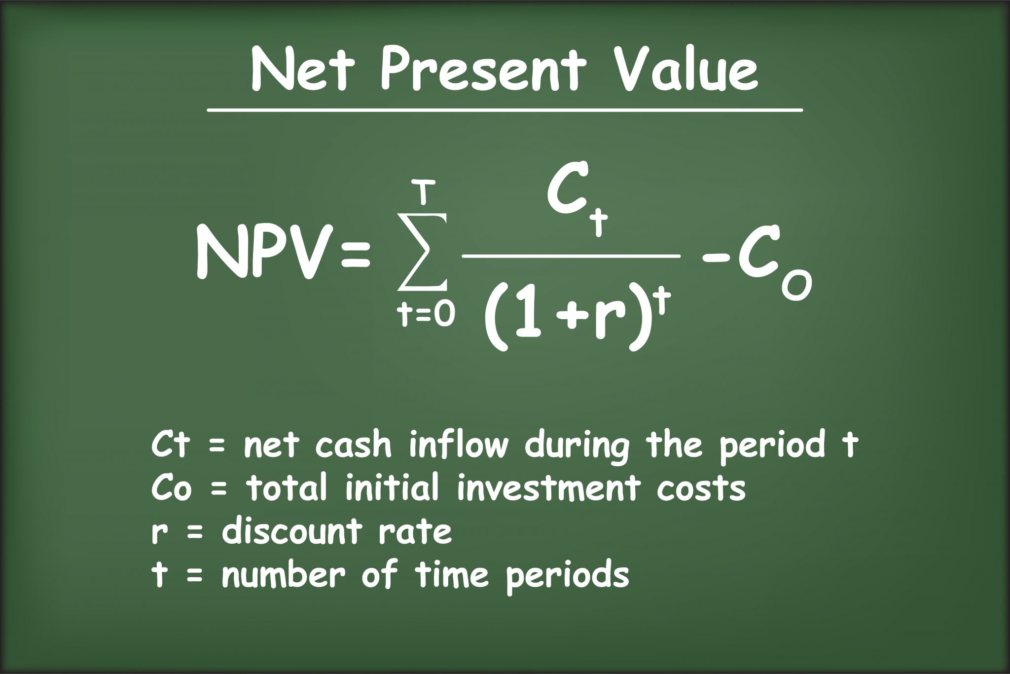
In engineering economics and corporate finance, Net Present Worth (NPW) serves as a fundamental metric for determining the value of an investment in today's dollars. However, a significant analytical error occurs when a decision-maker compares two mutually exclusive alternatives that do not share the same service life. For example, if you are choosing between a piece of equipment that lasts three years and one that lasts five years, the five-year asset naturally accumulates more costs and revenues simply because it operates longer.
A direct NPW comparison over different horizons is "apples-to-oranges" because it ignores what happens after the shorter-lived asset expires. To make a valid "apples-to-apples" comparison, the analysis must account for the continued service required after the first asset's life ends. As of 2026, standard financial reporting and capital budgeting protocols strictly require normalized comparison periods to avoid skewed Return on Investment (ROI) projections.
The primary assumption used in these comparisons is the Repeatability Assumption. This assumes that when a project’s life ends, an identical replacement can be purchased with the same costs and benefits. If this assumption does not hold—perhaps due to rapidly changing technology or fluctuating market conditions—the analyst must instead use a fixed Study Period or Planning Horizon.
Method 1: The Least Common Multiple (LCM) of Lives
The Least Common Multiple (LCM) method is the traditional approach to resolving the "2 lives" problem. By finding the smallest number of years into which both project lives can be divided evenly, you create a common terminal point for the analysis.
How the LCM Method Works
If Project A has a life of 2 years and Project B has a life of 3 years, the LCM is 6 years. To perform the comparison:
- Project A (2-year life): Assume the project is repeated three times (2 + 2 + 2 = 6 years). The initial investment cost is incurred at Year 0, Year 2, and Year 4.
- Project B (3-year life): Assume the project is repeated twice (3 + 3 = 6 years). The initial investment cost is incurred at Year 0 and Year 3.
- Discounting: Discount all cash flows (revenues, operating costs, and replacement costs) back to Year 0 using the Minimum Attractive Rate of Return (MARR).
- Comparison: Compare the total NPW of both projects over the 6-year period. The one with the higher NPW (or lower Net Present Cost) is the preferred alternative.
Constraints of the LCM Method
While mathematically sound, the LCM method can become cumbersome if the lifespans are large or prime numbers. For instance, comparing a 7-year asset with an 11-year asset requires a 77-year study period. In the 2026 economic landscape, projecting costs 77 years into the future is often viewed as speculative and unreliable. In such cases, the Equivalent Annual Worth method is generally preferred.

Method 2: Equivalent Annual Worth (EAW)
The Equivalent Annual Worth (EAW) method—also known as Equivalent Annual Cost (EAC) when dealing only with expenses—is often the most efficient way to handle the "2 lives" discrepancy. Instead of expanding the timeframe to a common multiple, this method converts the NPW of each alternative into a uniform annual series of payments over its respective life.
The Mathematical Logic
The EAW calculates the "annualized" value of an investment. Because it represents a yearly average that accounts for the time value of money, the EAW of a 3-year project can be directly compared to the EAW of a 5-year project.
To calculate EAW, you first find the NPW of a single cycle of the project, then multiply it by the Capital Recovery Factor (CRF):
EAW = NPW × [ (i(1+i)^n) / ((1+i)^n - 1) ]
Where:
- i = Discount rate (MARR)
- n = Service life of the specific alternative
Why EAW is Dominant in 2026
In modern financial modeling, EAW is favored because it avoids the need to explicitly map out multiple replacement cycles. It inherently assumes the project will be repeated indefinitely or at least long enough that the differences in life no longer matter. It is particularly useful for assets that are part of a continuous operation, such as manufacturing machinery or fleet vehicles.
Method 3: The Fixed Study Period (Planning Horizon)
There are instances where neither the LCM nor the EAW method is appropriate. This occurs when a project is tied to a specific contract length or a company’s strategic window. If a firm intends to exit a specific market in exactly 5 years, it does not matter if a machine lasts 3 years or 10 years; the analysis must be constrained to that 5-year Study Period.
Handling the Shorter Life
If the study period is 5 years and the asset lasts only 3 years, the analyst must include the cost of a replacement or a rental for the remaining 2 years. This is common in 2026 infrastructure projects where "bridge" solutions are used to fill gaps in service.
Handling the Longer Life
If the asset lasts 10 years but the study period is only 5, the analyst must calculate the Terminal Value or Salvage Value of the asset at the end of Year 5. This represents the remaining economic value of the machine that could be recovered by selling it or repurposing it elsewhere. This value is then discounted back to Year 0 and added to the NPW.
Comparison of Methods for Unequal Lives
The following table summarizes the three primary approaches to comparing two projects with different lifespans.
| Feature | Least Common Multiple (LCM) | Equivalent Annual Worth (EAW) | Fixed Study Period |
|---|---|---|---|
| Primary Use Case | When repeatability is certain and lives are small. | When comparing continuous operations or long lives. | When a specific business deadline exists. |
| Assumption | Assets are replaced with identical versions. | Assets are replaced with identical versions indefinitely. | Assets are sold or supplemented at a specific date. |
| Calculation Complexity | High (requires multiple cycles of cash flows). | Low (uses a single formula/factor). | Moderate (requires terminal value estimates). |
| Timeframe | Variable (LCM of both lives). | 1 Year (Annualized). | Fixed (Defined by the user). |
| Decision Rule | Choose the highest NPW over the LCM period. | Choose the highest EAW. | Choose the highest NPW over the fixed period. |
Step-by-Step Calculation Guide: LCM Method
To illustrate the practical application of the "2 lives" problem, consider two machines being evaluated for a production line in 2026. The company’s MARR is 10%.
- Machine A: Costs $20,000, lasts 2 years, salvage value $0, annual benefit $15,000.
- Machine B: Costs $30,000, lasts 3 years, salvage value $5,000, annual benefit $15,000.
Step 1: Determine the LCM
The LCM of 2 and 3 is 6 years.
Step 2: Map Cash Flows for Machine A (3 Cycles)
- Year 0: -$20,000 (Initial cost)
- Year 1: +$15,000
- Year 2: +$15,000 - $20,000 (Benefit minus replacement cost) = -$5,000
- Year 3: +$15,000
- Year 4: +$15,000 - $20,000 (Benefit minus replacement cost) = -$5,000
- Year 5: +$15,000
- Year 6: +$15,000
Step 3: Map Cash Flows for Machine B (2 Cycles)
- Year 0: -$30,000 (Initial cost)
- Year 1: +$15,000
- Year 2: +$15,000
- Year 3: +$15,000 - $30,000 + $5,000 (Benefit minus replacement plus salvage) = -$10,000
- Year 4: +$15,000
- Year 5: +$15,000
- Year 6: +$15,000 + $5,000 (Benefit plus final salvage) = +$20,000
Step 4: Calculate Present Worth
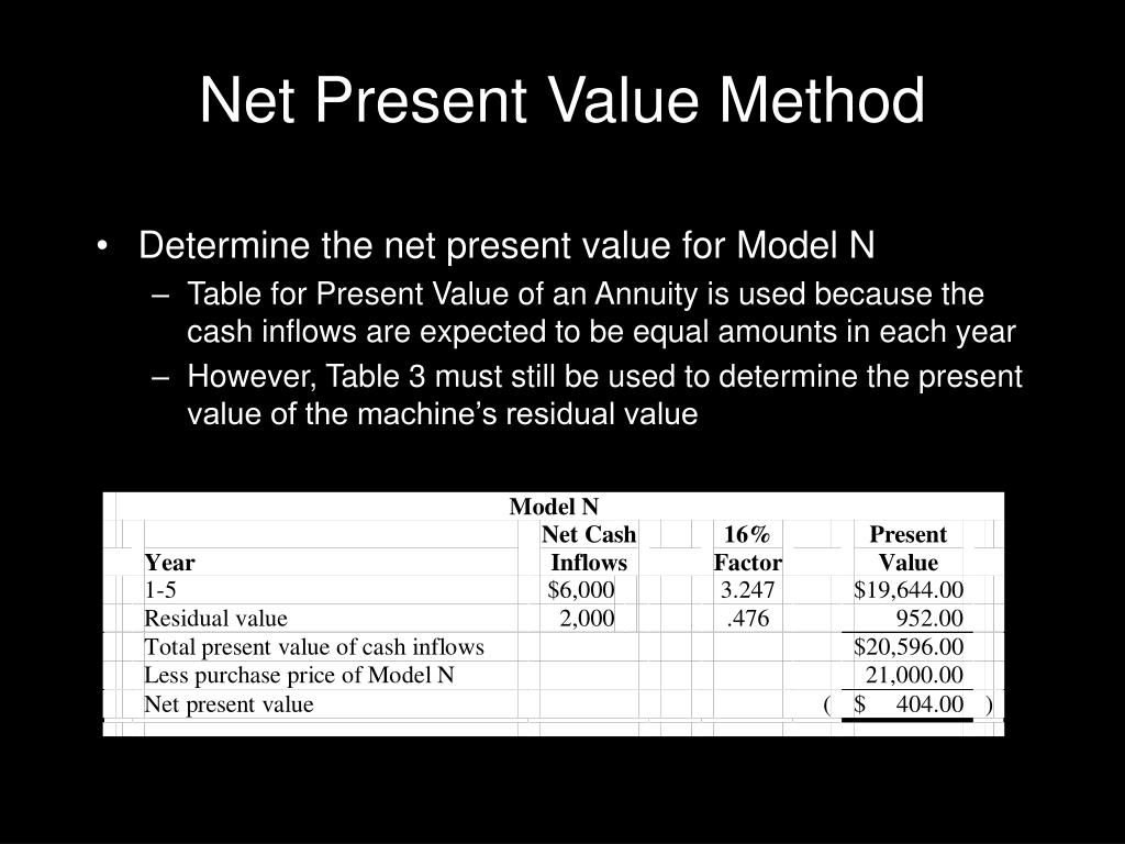
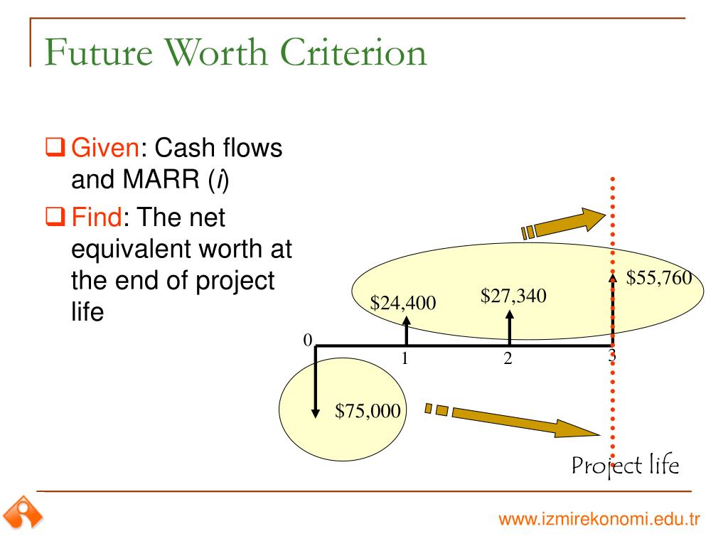
Discount all these flows back to Year 0 at 10%. The machine with the higher total present value over the 6-year horizon is the winner. This process accounts for the fact that Machine A must be purchased more frequently than Machine B.
Key Considerations and Potential Pitfalls
Inflation and Cost Escalation
In the year 2026, economists emphasize that the "Identical Replacement" assumption is often flawed. If you are using the LCM method, you must consider whether the cost of Machine A will still be $20,000 in Year 2 and Year 4. If inflation or technological advancements change the price, those adjustments must be built into the cash flow model.
The Impact of the Discount Rate
The choice of the discount rate (MARR) significantly affects projects with unequal lives. A higher discount rate penalizes future cash flows more heavily. Since shorter-lived projects require replacement capital sooner, a high interest rate environment may make longer-lived assets (which delay replacement) more attractive, even if their initial cost is higher.
Opportunity Costs
When assets have unequal lives, there is an inherent opportunity cost regarding the capital tied up in the more expensive, longer-lived asset. The EAW method is particularly good at capturing this because the Capital Recovery Factor includes both the recovery of the initial investment and the interest on the unrecovered balance.
Practical Expert Guidance for 2026
When tasked with comparing "2 lives," follow this hierarchy of decision-making:
- Check for a Study Period: Does the company have a specific timeframe for this project? If yes, use the Fixed Study Period method. Calculate salvage values for any equipment that outlasts the period.
- Evaluate for Repeatability: Is it likely that the equipment will be replaced by a similar model at a similar price?
- If yes, and the lives are small (e.g., 2 and 3, or 3 and 4), use the LCM Method. It is the most transparent for stakeholders to visualize.
- If yes, but the lives are large or odd (e.g., 7 and 13), use the EAW Method. It is mathematically cleaner and less prone to manual spreadsheet errors.
- Sensitivity Analysis: Always run the calculation at a slightly higher and lower MARR. If the "winner" changes based on a 1% shift in interest rates, the decision carries high risk and requires further qualitative analysis.
Frequently Asked Questions
Can I just use the NPW of a single life for each project?
No. Using the NPW of a single life for projects with unequal lives is a common mistake. It ignores the fact that the shorter project will end sooner, leaving you with no service or necessitating an immediate replacement that hasn't been factored into the costs. This usually makes the shorter-lived project look unfairly better because its long-term replacement costs are hidden.
Which method is more accurate: LCM or EAW?
Both are mathematically equivalent if the same assumptions (repeatability and constant costs) are used. EAW is generally considered more "practical" in 2026 because it is easier to calculate and explain to non-technical stakeholders as an "annualized cost." However, LCM is more "accurate" if you know for a fact that costs will change specifically at each replacement interval.
How do I handle salvage value in unequal life comparisons?
Salvage value should be included at the end of every life cycle. In the LCM method, if an asset has a salvage value, you subtract it from the cost of the replacement asset in those years where a cycle ends and a new one begins (except for the very last year, where it is simply a cash inflow). In the EAW method, the salvage value is converted to an equivalent annual credit using the Sinking Fund Factor.
What if the two projects have completely different functions?
NPW comparison for unequal lives is only valid for mutually exclusive alternatives that provide the same service. If the projects serve different purposes or have different revenue-generating capabilities that aren't comparable, NPW alone is insufficient. You would likely need to look at a broader Benefit-Cost Ratio (BCR) or Internal Rate of Return (IRR) analysis.
Is the "2 lives" problem relevant for software subscriptions?
In 2026, most software is SaaS-based (Software as a Service), meaning it is essentially an infinite-life service with annual payments. The unequal life problem is most relevant for physical infrastructure, hardware, and manufacturing equipment where there is a heavy upfront "sunk" cost followed by a period of use and eventually a required replacement.
Final Recommendation
When comparing "net present worth 2 lifes," prioritize the Equivalent Annual Worth (EAW) method. It simplifies the mathematical burden by standardizing the comparison to a single year, automatically accounting for the discrepancy in project lifespans without the need to project cash flows over decades. For 2026 capital budgeting, EAW provides a clearer, more defensible metric for stakeholders while maintaining full integrity regarding the time value of money.
Image Gallery
Select an image to open it in a new tab.



Ingrid Bjornson
Global Cyber Policy and Regulation Analyst
