The Davies-Bouldin Score for Cluster Validation: A Comprehensive Guide
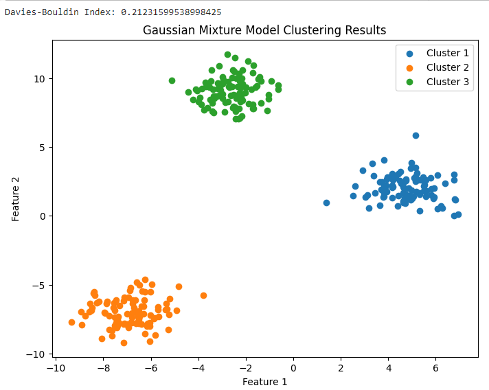
The Davies-Bouldin score is an internal evaluation metric used to assess the quality of clustering algorithms by measuring the average similarity between each cluster and its most similar peer. A lower Davies-Bouldin score indicates a better clustering result, signifying that the clusters are compact and well-separated from one another.
In the field of unsupervised machine learning, determining the "goodness" of a model is inherently difficult because there are no ground-truth labels to compare against the predictions. Unlike supervised learning, where we can calculate accuracy or F1-scores against known targets, clustering requires internal validation metrics that analyze the structure of the data itself. The Davies-Bouldin Index (DBI) has remained a cornerstone of this evaluation process for decades, providing a mathematical framework to quantify how well a dataset has been partitioned into distinct groups.
The Role of Cluster Validation in 2026 Machine Learning
As of 2026, data science workflows have become increasingly automated through AutoAI and MLOps pipelines. However, the fundamental need for robust validation metrics remains unchanged. When an algorithm like K-Means, Bisecting K-Means, or Gaussian Mixture Models partitions a dataset, we need a way to answer a critical question: Is this specific number of clusters (k) optimal for the underlying data structure?
Cluster validation techniques are generally categorized into two types: external and internal. External validation requires a "gold standard" or pre-labeled dataset, which is rarely available in real-world exploratory data analysis. Internal validation, where the Davies-Bouldin score resides, uses only the information present in the data. It evaluates the results based on two primary criteria:
- Cohesion (Compactness): How closely related the objects in the same cluster are. We want the points within a group to be as tight as possible around a central point.
- Separation: How distinct or well-spaced the different clusters are from each other. We want a clear "no man's land" between different groups to prevent overlap.
The Davies-Bouldin score is particularly valued because it offers a balanced ratio of these two factors, providing a single numerical value that is easy to interpret and optimize during hyperparameter tuning.
Mathematical Foundation of the Davies-Bouldin Index
To truly understand the Davies-Bouldin score for cluster validation, one must look at the mechanics of its calculation. The index is defined as the average similarity between each cluster and its "most similar" neighbor. The logic follows a step-by-step aggregation of dispersion and distance.
1. Measuring Cluster Scatter (S_i)
For every cluster, we calculate a scatter value, often denoted as S_i. This is typically the average distance between all points in the cluster and the centroid of that cluster. If the points are tightly packed around the center, S_i will be small. If the cluster is diffuse or stretched out, S_i will be large. Mathematically, this represents the internal variance of the group.
2. Measuring Separation Between Clusters (M_ij)
Next, we look at the distance between the centroids of two different clusters, i and j. This is denoted as M_ij. This value measures how far apart the "hearts" of the clusters are. In most implementations, Euclidean distance is used for this calculation, though other Minkowski metrics can be applied depending on the data type.
3. Calculating the Similarity Ratio (R_ij)
The core of the Davies-Bouldin logic lies in the ratio R_ij. This is calculated as:
R_ij = (S_i + S_j) / M_ij
This formula essentially asks: "Compared to how far apart these two clusters are (M_ij), how much space do they take up (S_i + S_j)?"
- If the sum of their scatters is much smaller than the distance between them, the ratio is low, indicating the clusters are well-separated.
- If the sum of their scatters is large compared to the distance between them, the ratio is high, indicating that the clusters are either very sparse or overlapping.
4. Selecting the Maximum Similarity (D_i)
For each cluster i, the algorithm finds the maximum value of R_ij for all other clusters j. This identifies the "worst-case scenario" for cluster i—its closest or most confusing neighbor. We denote this maximum value as D_i.
5. The Final Davies-Bouldin Index
The final DBI is the arithmetic mean of all the D_i values across all clusters in the model. Because the index is an average of "worst-case" similarities, a lower overall score represents a model where even the most similar clusters are still reasonably distinct and compact.
Step-by-Step Execution of the Validation Process
When applying the Davies-Bouldin score for cluster validation in a technical environment, the workflow generally follows these stages:
Data Preprocessing and Scaling Because the Davies-Bouldin score relies heavily on Euclidean distances, it is sensitive to the scale of the features. If one feature (like "Annual Income") has a range in the thousands and another (like "Age") ranges from 1 to 100, the income feature will dominate the distance calculation. Before calculating the DBI, it is essential to perform standard scaling or normalization to ensure each feature contributes equally to the scatter and separation metrics.
Clustering Implementation
You must first run a clustering algorithm on your dataset. Let’s assume you are using K-Means. You would typically run the algorithm for a range of possible cluster counts—for example, k=2 through k=10.
Calculating the DBI for Each Model
For each resulting set of clusters, you calculate the Davies-Bouldin score. In modern software environments, this is usually handled by built-in functions, such as davies_bouldin_score in Python’s Scikit-Learn library.
Analysis and Optimization
You plot the number of clusters on the x-axis and the DBI on the y-axis. Unlike the "Elbow Method" used with Within-Cluster Sum of Squares (WCSS), where you look for a bend in the curve, with DBI you are looking for the global minimum. The value of k that yields the lowest Davies-Bouldin score is mathematically suggested as the most appropriate number of clusters for that specific dataset.
Interpreting the Davies-Bouldin Score Results
Interpreting the score requires an understanding of its bounds. The score is non-negative, with a theoretical lower bound of zero.
| Score Range | Interpretation | Suggested Action |
|---|---|---|
| Near 0.0 | Perfect separation. This usually only occurs in synthetic datasets or perfectly distinct groups. | Highly confident in cluster structure. |
| 0.0 - 0.5 | Excellent clustering. The clusters are very compact and far apart from one another. | Model is likely optimal. |
| 0.5 - 1.2 | Good to Moderate. Some clusters might be close, but they are generally well-defined. | Standard result for real-world noisy data. |
| 1.2 - 2.0 | Fair to Weak. Clusters are starting to overlap significantly or are very spread out. | Consider changing the number of clusters or the feature set. |
| Above 2.0 | Poor validation. The clusters are likely poorly defined or the data does not have a natural centroid-based structure. | Re-evaluate the algorithm choice or data preprocessing. |
It is important to note that the "ideal" score is relative to the specific dataset. In highly complex biological or financial data, a score of 1.5 might be the best possible outcome, whereas, in simple customer segmentation, you might expect a score below 1.0.
Comparing Davies-Bouldin to Other Validation Metrics
While the Davies-Bouldin score is a powerful tool, it is rarely used in isolation. It is most effective when compared against other internal validation metrics like the Silhouette Coefficient and the Calinski-Harabasz Index.
Davies-Bouldin vs. Silhouette Coefficient
The Silhouette Coefficient measures how similar an object is to its own cluster compared to other clusters. The scores range from -1 to +1. While the Silhouette score is often more intuitive (higher is better), it is computationally more expensive than DBI because it requires calculating the distance between every pair of points. The Davies-Bouldin score only requires calculating distances between points and centroids and then between the centroids themselves, making it much faster for very large datasets.
Davies-Bouldin vs. Calinski-Harabasz Index
The Calinski-Harabasz Index (also known as the Variance Ratio Criterion) is the ratio of the sum of between-clusters dispersion and of within-cluster dispersion. Unlike DBI, where lower is better, for Calinski-Harabasz, a higher score is better. Calinski-Harabasz is generally even faster than DBI but can be overly sensitive to the number of data points, sometimes favoring higher cluster counts disproportionately.
Practical Advantages of the Davies-Bouldin Score
The Davies-Bouldin score for cluster validation offers several distinct advantages that keep it relevant in 2026's data-driven landscape:
- Computational Efficiency: As mentioned, it focuses on centroids. In an era where datasets frequently contain millions of rows, calculating point-to-point distances (as the Silhouette score does) can be prohibitive without significant downsampling. DBI scales much better for large-scale production environments.
- Simplicity of Interpretation: Having a score where the goal is minimization aligns naturally with many optimization algorithms used in machine learning.
- Intuitive Logic: The idea of "Scatter vs. Separation" is easy to explain to non-technical stakeholders. It mirrors the human visual perception of what makes a "good" group—items that are close together but far from other things.
- Boundedness: Because the score cannot be negative, it provides a clear floor for optimization, preventing the confusion that can sometimes arise with metrics that oscillate across zero.
Limitations and Critical Considerations
Despite its utility, the Davies-Bouldin score has limitations that a senior technical editor must highlight to ensure accurate application.
Assumptions of Convexity The Davies-Bouldin score is fundamentally a centroid-based metric. This means it assumes that clusters should be spherical or convex. If your data contains clusters with complex, non-linear shapes (like interlocking crescents or spirals), DBI will likely give a poor score even if the clustering algorithm (like DBSCAN or Spectral Clustering) has correctly identified the patterns. In these cases, density-based validation metrics are more appropriate.
Sensitivity to Distance Metrics The index is strictly tied to the distance metric used. If you use Euclidean distance on high-dimensional data, you may fall victim to the "curse of dimensionality," where the distance between any two points starts to look very similar. This can lead to compressed DBI scores that fail to distinguish between good and bad models.
The Minimum at k=1
The formula for DBI is typically not defined for k=1 (since there are no other clusters to compare against). However, it is a known behavior that in some implementations, the score might improve as k increases simply because the scatter (S_i) decreases as clusters get smaller. It is vital to look for a clear, significant minimum rather than just selecting the highest possible k.
Implementing the Score in Modern Workflows
In 2026, the Davies-Bouldin score is integrated into most automated machine learning (AutoML) frameworks. When building a pipeline, the validation step acts as a "gatekeeper."
For example, a typical Python-based workflow would look like this:
- Import
davies_bouldin_scorefromsklearn.metrics. - Initialize a list to store scores.
- Loop through values of
k(e.g., 2 to 15). - Fit the model and predict labels.
- Pass the data and labels to the
davies_bouldin_scorefunction. - Identify the index of the minimum score.
This process allows for "hands-off" optimization where the system can automatically select the best configuration for a clustering task before passing the results to a downstream application, such as a personalized recommendation engine or an anomaly detection system.
Common Mistakes to Avoid
- Ignoring Feature Scaling: As emphasized, the reliance on centroids and Euclidean distance makes scaling non-negotiable. Skipping this step renders the DBI meaningless.
- Relying Solely on DBI: No single metric is perfect. A low DBI might suggest great clusters that are actually irrelevant to the business problem. Always pair internal validation with a qualitative "sanity check" of the resulting groups.
- Using DBI for Density-Based Algorithms: If you are using DBSCAN or OPTICS to find clusters of varying densities and shapes, DBI will likely penalize the model unfairly. Use DBI primarily for partition-based algorithms like K-Means or K-Medoids.
- Over-optimizing for the Score: Sometimes, a slightly higher DBI score results in clusters that are more "interpretable" or "actionable" for human users. The goal of data science is often utility, not just mathematical perfection.
Frequently Asked Questions
Is a lower Davies-Bouldin score always better?
Mathematically, yes. A lower score indicates that the clusters are more compact and better separated. However, it must be viewed in context; if a lower score is achieved by creating an impractical number of clusters (e.g., 50 clusters for a small dataset), the model may be overfitting the noise rather than finding meaningful patterns.
Can the Davies-Bouldin score be used for categorical data?
Standard DBI is designed for continuous numerical data where centroids and Euclidean distances are meaningful. To use it for categorical data, you must first transform the data using techniques like Multiple Correspondence Analysis (MCA) or use a modified version of the index that supports Gower’s distance or other categorical similarity measures.
How does DBI handle noise and outliers?
The Davies-Bouldin score is relatively sensitive to outliers. Because outliers increase the "scatter" (the average distance to the centroid), a few well-placed outliers can significantly inflate the DBI score, making a good clustering result look poor. It is often recommended to perform outlier detection and removal before validation.
Does the Davies-Bouldin score work with hierarchical clustering?
Yes. Once the hierarchical clustering is "cut" at a specific level to produce a fixed number of clusters, the DBI can be calculated for that specific partition. This is a common way to decide at what height to cut a dendrogram.
What is the difference between DBI and the Elbow Method?
The Elbow Method uses the "Sum of Squared Errors" (SSE) within clusters. It looks for a point where adding more clusters no longer provides a significant decrease in SSE. DBI is more sophisticated because it considers both internal tightness AND the distance between groups, whereas the Elbow Method only looks at internal tightness.
Why is the Davies-Bouldin score preferred over the Silhouette score for large datasets?
The primary reason is computational complexity. The Silhouette score requires $O(N^2)$ distance calculations, where $N$ is the number of samples. The Davies-Bouldin score primarily relies on the number of clusters ($k$) and the number of samples ($N$), scaling roughly at $O(N \cdot k)$. When $N$ is in the millions, DBI is significantly faster to compute.
Practical Recommendation
When using the Davies-Bouldin score for cluster validation, always start by standardizing your features to a zero mean and unit variance. Run your clustering algorithm across a range of k values and identify the point where the DBI reaches its first significant local minimum. To ensure the highest level of model integrity, cross-validate this result by checking the Silhouette Coefficient and the Calinski-Harabasz Index. If all three metrics point to the same number of clusters, you can be highly confident in the stability and validity of your model. If they disagree, prioritize the metric that best aligns with your data's geometry (e.g., use DBI for spherical clusters and Silhouette for more varied shapes).
Image Gallery
Select an image to open it in a new tab.
Vivian Cho
Executive IT and Emerging Technologies Reporter
