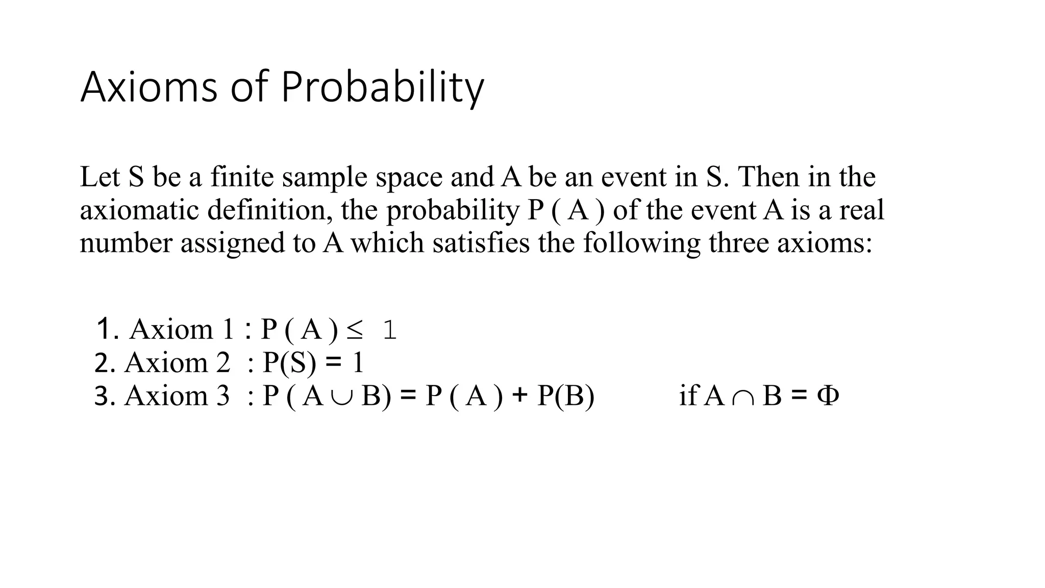
The probability axioms are a set of three fundamental rules, established by Andrey Kolmogorov in 1933, that provide the mathematical framework for all probability theory. These axioms—non-negativity, normalization, and countable additivity—ensure that probability functions consistently across both simple discrete outcomes and complex, infinite continuous systems within modern measure theory.
Probability is often perceived as a tool for gambling or weather forecasting, but in the scientific landscape of 2026, it serves as the backbone of artificial intelligence, quantum mechanics, and financial risk modeling. To understand how we calculate the likelihood of an event, we must look beyond intuition and toward the formal structures known as the Kolmogorov Axioms. These axioms do not tell us what the probability of a specific event is; rather, they define the rules that any valid probability measure must follow.
The Evolution of Probability: From Heuristics to Axioms
Before the early 20th century, probability was largely treated as a branch of applied mathematics focused on games of chance. The "Classical Definition," popularized by Pierre-Simon Laplace, suggested that the probability of an event was simply the ratio of favorable outcomes to the total number of equally likely outcomes. While this worked for rolling dice or drawing cards, it failed when dealing with infinite sets or non-uniform distributions.
The need for a more rigorous approach became evident as physics and economics began demanding more complex models. In 1933, Russian mathematician Andrey Kolmogorov published Foundations of the Theory of Probability. He realized that probability could be treated as a special type of "measure," a concept from the mathematical field of measure theory. By anchoring probability in set theory, Kolmogorov provided a universal language that remains the standard in 2026.
The Fundamental Building Blocks: The Probability Triple
Before we examine the axioms themselves, we must define the environment in which they operate. Mathematicians describe a probability space as a "triple" consisting of three components: $(\Omega, \mathcal{F}, P)$.
1. The Sample Space ($\Omega$)
The sample space, denoted by the Greek letter Omega ($\Omega$), is the set of all possible outcomes of a random experiment. For a coin toss, $\Omega = {\text{Heads, Tails}}$. In 2026's data science applications, $\Omega$ might represent millions of potential configurations of a neural network's weights.
2. The Sigma-Algebra ($\mathcal{F}$)
This is often the most difficult concept for students to grasp. The sigma-algebra is a collection of subsets of the sample space. An "event" is an element within $\mathcal{F}$. For the axioms to hold, $\mathcal{F}$ must be closed under complements and countable unions. This ensures that if we can talk about the probability of "rain," we can also mathematically define the probability of "not rain."
3. The Probability Measure ($P$)
$P$ is a function that assigns a real number to every event in the sigma-algebra $\mathcal{F}$. The axioms are the constraints placed upon this function $P$.
The Three Axioms of Kolmogorov
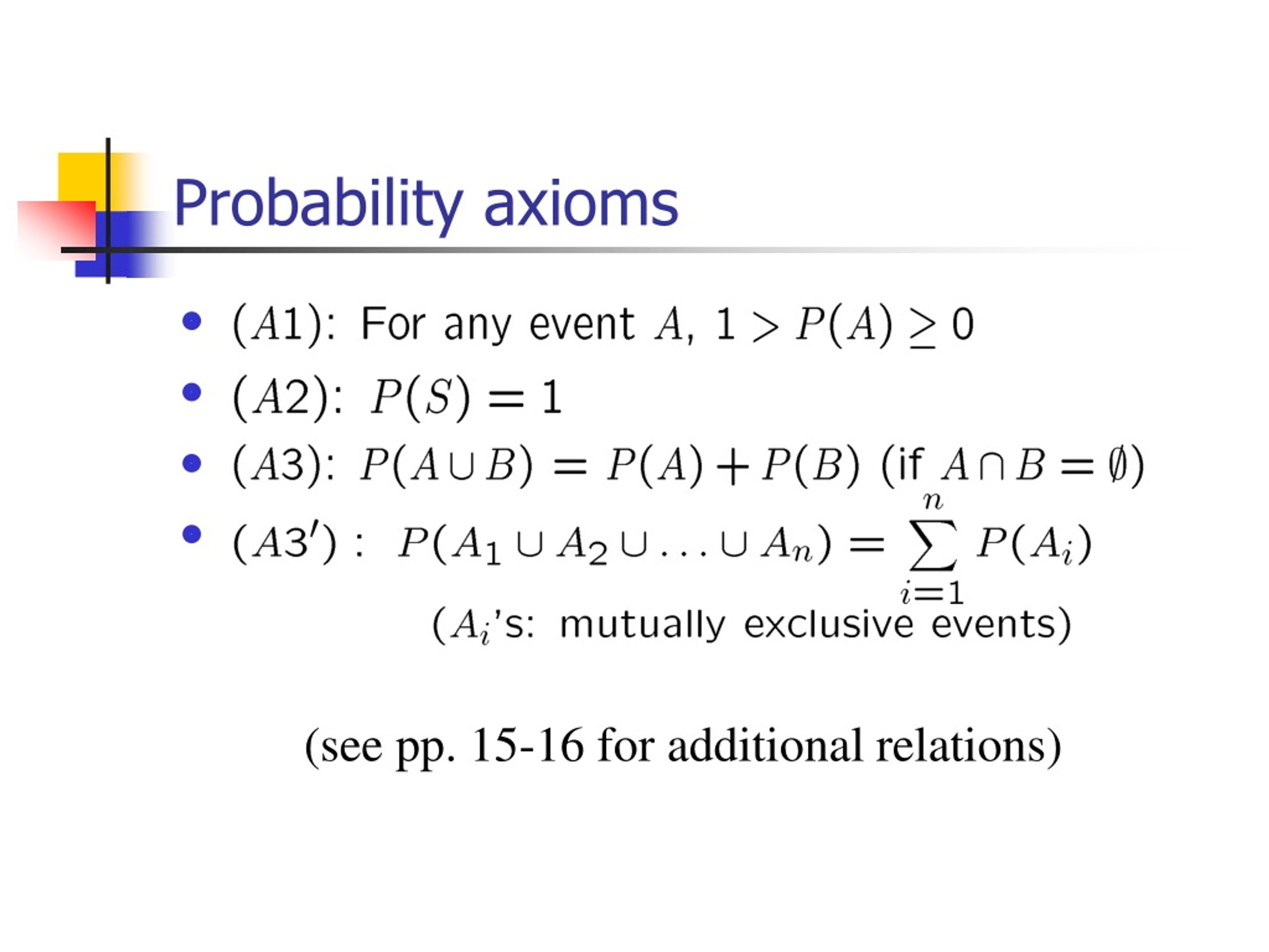
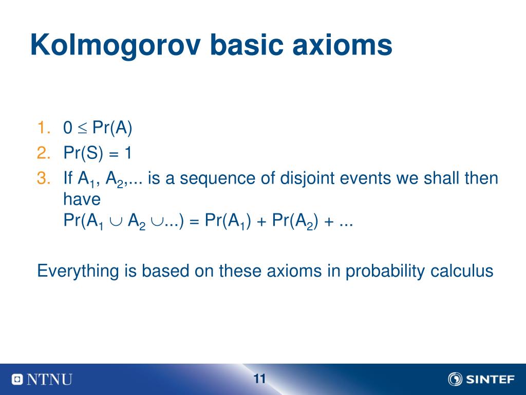
The beauty of Kolmogorov's work lies in its simplicity. From just three rules, the entire complexity of modern statistical inference is derived.
Axiom 1: Non-Negativity
For any event $A$, $P(A) \ge 0$.
This axiom states that probability can never be a negative number. While this seems intuitive—you cannot have a -20% chance of an event occurring—it is a vital formal constraint. In mathematical terms, this establishes that the probability measure is a "mapping" from the set of events to the interval of non-negative real numbers. If a calculation results in a negative value, the model is fundamentally flawed or does not represent a valid probability space.
Axiom 2: Normalization (Unit Measure)
The probability of the entire sample space is exactly one: $P(\Omega) = 1$.
This axiom defines the scale of probability. It asserts that something within the sample space must happen. If you roll a six-sided die, the probability that the result is either 1, 2, 3, 4, 5, or 6 is exactly 1 (or 100%). This provides the "ceiling" for our measurements. Without normalization, we could not compare different probability spaces, as their scales would be arbitrary.
Axiom 3: Countable Additivity
If $A_1, A_2, A_3, \dots$ is a sequence of mutually exclusive (disjoint) events, then $P(\cup_{i=1}^{\infty} A_i) = \sum_{i=1}^{\infty} P(A_i)$.
This is the most powerful of the three axioms. It states that if two or more events cannot happen at the same time (they are disjoint), the probability of at least one of them occurring is the sum of their individual probabilities. Kolmogorov specifically specified countable additivity, allowing this rule to apply to infinite sequences of events, which is essential for continuous probability and advanced calculus.
Derived Properties and Theorems
The axioms are the "laws" of the system, but the "tools" we use daily are derived from them. By applying these three rules, we can prove several essential properties used in 2026’s statistical software and algorithmic trading.
The Complement Rule
Since $P(\Omega) = 1$, and an event $A$ and its complement $A^c$ (not $A$) together make up the entire sample space, we can derive that $P(A^c) = 1 - P(A)$. This is foundational for calculating the probability of "at least one" success in a series of trials.
The Probability of the Empty Set
From the axioms, we can mathematically prove that the probability of the empty set (an impossible event) is zero: $P(\emptyset) = 0$. While intuitive, the formal proof relies on the fact that the empty set is the complement of the entire sample space $\Omega$.
The Addition Law for Non-Disjoint Events
The third axiom only applies to disjoint events. However, for events that can overlap (like "drawing a red card" and "drawing a King"), we use the derived formula: $P(A \cup B) = P(A) + P(B) - P(A \cap B)$. This prevents "double-counting" the overlap (the King of Hearts, in this example).
Comparison of Probability Frameworks
While the Kolmogorov Axioms are the gold standard, they are applied differently depending on the interpretation of "probability."
| Feature | Classical Probability | Frequentist Probability | Bayesian Probability | Axiomatic (Kolmogorov) |
|---|---|---|---|---|
| Source of Truth | Equal likelihood of outcomes | Long-run relative frequency | Degree of belief/Certainty | Mathematical measure theory |
| Handling Infinity | Poor/Limited | Requires limit theorems | Subjective priors | Rigorous via $\sigma$-additivity |
| Main Use Case | Basic games (dice, coins) | Clinical trials, A/B testing | Machine Learning, AI | Theoretical Foundations |
| Constraint | Outcomes must be finite | Requires repeatable trials | Requires a prior distribution | Must satisfy the 3 axioms |
Technical Depth: Why Sigma-Additivity Matters
A common question among students is why Axiom 3 requires "countable" additivity instead of just "finite" additivity. If we only had finite additivity, we could sum the probabilities of a fixed number of events (like 10 or 1,000). However, modern physics and finance deal with continuous variables—time, price, or distance.
In a continuous world, the probability of any single exact point (like a stock price being exactly $150.00000...$) is zero. To find the probability of a range, we must sum an infinite number of infinitesimal points. Countable additivity allows us to use integration (calculus) to calculate these probabilities. Without this specific wording in Kolmogorov’s third axiom, the transition from discrete probability (counting) to continuous probability (calculus) would have no formal mathematical justification.
Practical Applications in 2026
In the current year 2026, the axiomatic foundation of probability is more relevant than ever due to the ubiquity of high-dimensional data.
- Generative AI: Large Language Models (LLMs) function by calculating the probability of the "next token." These models must adhere to the normalization axiom to ensure that the sum of all possible next-word probabilities equals exactly one, allowing the model to choose the most likely path.
- Quantum Computing: Quantum mechanics is inherently probabilistic. The "Born Rule" in physics, which predicts the likelihood of a particle being in a certain state, must satisfy the Kolmogorov axioms to be considered a valid physical theory.
- Risk Management: In the financial sector, "Value at Risk" (VaR) models use these axioms to ensure that the total risk profile of a portfolio is mathematically sound, preventing the calculation of "impossible" probabilities during market volatility.
Common Pitfalls and Misunderstandings
Despite their simplicity, the axioms are often misapplied in both academic and professional settings.
- Confusing Mutually Exclusive with Independent: Axiom 3 applies to mutually exclusive events (events that cannot happen together). It does not apply to independent events (where one event doesn't affect the other). Adding the probabilities of two independent events that are not mutually exclusive will result in a value greater than 1, violating Axiom 2.
- Ignoring the Sample Space: Many errors arise from a poorly defined $\Omega$. If the sample space does not contain every possible outcome, the normalization axiom cannot be satisfied, rendering all subsequent calculations invalid.
- The "Zero-Probability" Paradox: In continuous probability, an event can have a probability of 0 without being impossible. For instance, picking a specific real number between 0 and 1 has a probability of 0, yet some number must be picked. This is a nuance of measure theory that the axioms accommodate through the sigma-algebra.
Frequently Asked Questions
Can a probability ever be greater than 1?
No. According to the second axiom (Normalization), the probability of the entire sample space $\Omega$ is 1. Since any event $A$ is a subset of $\Omega$, its probability $P(A)$ cannot exceed $P(\Omega)$. If a calculation results in a number greater than 1, it usually indicates that the events being summed are not mutually exclusive, leading to double-counting.
Who is Andrey Kolmogorov?
Andrey Kolmogorov was a Soviet mathematician who made significant contributions to various fields, including topology, turbulence, and logic. His 1933 monograph, Grundbegriffe der Wahrscheinlichkeitsrechnung (Foundations of the Theory of Probability), is credited with placing probability on a rigorous mathematical footing by linking it to measure theory.
What is the difference between an outcome and an event?
An outcome is a single result of an experiment (a "point" in the sample space). An event is a set of outcomes (a subset of the sample space). For example, in a die roll, "rolling a 4" is an outcome, while "rolling an even number" is an event consisting of the outcomes ${2, 4, 6}$. The axioms are defined in terms of events.
Why do we need the Sigma-Algebra ($\mathcal{F}$)?
The sigma-algebra is necessary because, in complex systems with infinite outcomes, it is sometimes mathematically impossible to assign a consistent probability to every possible subset. The sigma-algebra defines exactly which subsets are "measurable" (i.e., which subsets we are allowed to calculate probabilities for) to avoid logical paradoxes like the Banach-Tarski paradox.
How do these axioms relate to Bayesian statistics?
The Kolmogorov axioms are "engine-agnostic." Whether you are a Frequentist or a Bayesian, you must follow these axioms. The difference lies in how you determine the initial values (the inputs) for the probability measure $P$. Bayesians use the axioms to update their beliefs (priors) as new data arrives, but the underlying rules of $P$ remain the same.
Next Steps for Learning
To truly master the foundations of probability, one should move from the axioms into the study of Conditional Probability and Bayes' Theorem. These concepts explain how the probability of an event changes when we gain new information. Additionally, exploring Measure Theory will provide a deeper understanding of the "Lebesgue Integral," which is the advanced tool used to apply Kolmogorov's third axiom to continuous distributions.
For those working in data science or engineering in 2026, the next practical step is often learning how these axioms are implemented in computational libraries like Python’s SciPy or TensorFlow Probability, which automate the rigorous requirements of the axioms for complex datasets.
Image Gallery
Select an image to open it in a new tab.
Declan O'Connor
Higher Education and Campus Culture Reporter
